Revised image processing commands

imversion

Display version information

This command displays image library version information. Last modification date of an image library command can be retrieved using -version parameter.

General and I/O commands

imcreate	Create a new image
-n <name>	image name in NDA-namespace
-t <type>	image type [1=binary $\vert$ 2=int $\vert$ 3=real $\vert$ 4=complex]
-d <depth>	image depth (max. 32 bits)
-w <width>	image width in pixels
-h <height>	image height in pixels
[-ti <index>]	time index for animated images (default: 0)
[-ci <index>]	color index for spectral images (default: 0)
[-li <index>]	layer index for 3D images (default: 0)

This command creates a new image with selected type, size, and tags. An image can represent a (x,y)-plane of pixels (regular images) or (spectrum,angle)-plane (Fourier transformed images). Images can be combined to imagelists. Time index is used to define the position of the image in an animation. Color index is used to distinguish images taken from different areas of the color spectrum. Layer index is used for creating 3D voxel representations where images are stacked in piles.

imgettime	Get the time value from an image
-n <name>	image name
-v <value>	field name receiving the time value
imputtime	Put a time value to an image
-n <name>	image name
-v <value>	new value
imgetcolor	Get the color value from an image
-n <name>	image name
-v <value>	field name receiving the color value
imputcolor	Put a color value to an image
-n <name>	image name
-v <value>	new value
imgetlayer	Get the layer value from an image
-n <name>	image name
-v <value>	field name receiving the layer value
imputlayer	Put a layer value to an image
-n <name>	image name
-v <value>	new value

These commands provide a way to read and write image tags. For more information on tags please refer to imcreate above.

imgetpixel	Get a pixel value from an image
-n <name>	image name
-x <position>	horizontal pixel index
-y <position>	vertical pixel index
-v <name>	field name receiving the pixel value
imputpixel	Put a pixel value to an image
-n <name>	image name
-x <position>	horizontal pixel index
-y <position>	vertical pixel index
-v <value>	new value
imgetipixel	Get an imaginary pixel value from an image
-n <name>	image name
-x <position>	horizontal pixel index
-y <position>	vertical pixel index
-v <name>	field name receiving the pixel imaginary value
imputipixel	Put an imaginary pixel value to an image
-n <name>	image name
-x <position>	horizontal pixel index
-y <position>	vertical pixel index
-v <value>	new imaginary value

These commands offer a low-level access to image's bitplane. They offer only moderate performance and should not be used for laborious tasks. The imaginary versions of the commands are reserved for images where the pixels are complex numbers.

imconvert	Convert image to a new one
-src <name>	source name
-dest <name>	destination name
-t <type>	image type [1=binary $\vert$ 2=int $\vert$ 3=real $\vert$ 4=complex]
-d <depth>	image depth (max. 32 bits)

This command converts an existing image to a new one, which is of different type.

imsize	Get the size of an image
-n <name>	image name
-fout <size>	field name receiving the image size

This command inquires the pixel width and height of an image.

imcopy	Copy an image to another image
-src <name>	source name
-dest <name>	destination name

This command allows the user to make copies of images.

imload	Load an image from a file
-n <name>	image name
-f <filename>	filename (GIF-file)
[-ti <index>]	time index for animated images (default: 0)
[-ci <index>]	color index for spectral images (default: 0)
[-li <index>]	layer index for 3D images (default: 0)
imsave	Save an image into a file
-n <name>	image name
-f <filename>	filename (GIF-file)

These commands are used to load/save images from/to the filesystem. The only supported file format is CompuServe Graphics Interchange Format (*.gif).

Example: In this example we load and save an image from/to a file.

imload -n image -f paper.gif -ti 1 -ci 2 -li 0
imsave -n image -f img2.gif

Conversion commands

image2im	Convert an old image format to the new format
-src <name>	source name
-dest <name>	destination name
im2image	Convert an image from the new format to the old format
[
-gray <name>	source name for gray channel
$\vert$
-red <name>	source name for red channel
-green <name>	source name for green channel
-blue <name>	source name for blue channel
]
-dest <name>	destination name

These commands convert images from/to the old image format which is only required for visualization purposes.

Example: In this example we convert the image formats back and forth.

imload -n image -f paper.gif
im2image -gray image -dest oldimage
mkgrp g
bgimg g -img oldimage
show g
image2im -src oldimage -dest image2

Pixel-level commands

imhistogram	Builds a grayscale histogram
-src <name>	source name
-dest <name>	destination name
[-bits <name>]	histogram color model bit count (default is 8)

This command builds a histogram of the amounts of pixels of each gray intensity level in the image. Full-size 32-bit histogram has $2^{32}$ pins, which makes it impractical. Setting parameter -bits to lower value will generate histograms from $2^{bits}$ color model.

imconstraint	Set pixel values lower than lower bound and higher than upper bound to specified values
-src <name>	source name
-dest <name>	destination name
-t <type>	threshold type [1=lower $\vert$ 2=upper $\vert$ 3=both]
[
-lb <value>	24-bit lower threshold
-lv <value>	new 24-bit value for pixels below lower threshold
]
[
-ub <value>	24-bit upper threshold
-uv <value>	new 24-bit value for pixels above upper threshold
]

This command is used to make pixelwise thresholds directly to the image. Pixels, whose value is below the lower bound, are set to the lower value. Pixels whose intensity value is higher than the upper bound are set to the upper value. Intensity values are given in 24-bit format as NDA cannot store the full 32-bit format in it's namespace. In 24-bit model 0 is the lowest value (black) and 16777216 is the highest value (white).

imcrop	Crop a region from an image to another image
-src <name>	source name
-dest <name>	destination name
-x1 <position>	horizontal start pixel index
-y1 <position>	vertical start pixel index
-x2 <position>	horizontal end pixel index
-y2 <position>	vertical end pixel index

This command picks a subregion from an image to a new image.

imnegate	Negate the pixel values of an image and store them into another image
-src <name>	source name
-dest <name>	destination name

This command flips the gray intensities in order to make dark areas appear bright and vice versa.

imfilter	Filter an image
-src <name>	source name
-dest <name>	destination name
-o <operation>	mask operation [0=average $\vert$ 1=median]
-s <size>	mask size in pixels

This command applies a smoothing filter to the image.

imfindthreshold	Find a suitable threshold value from an image
-src <name>	source name
-m <mode>	operation mode [absolut $\vert$ percent $\vert$ mean $\vert$ median $\vert$ mode $\vert$ iterative $\vert$ otsu $\vert$ entropy $\vert$ entropy2 $\vert$ moment $\vert$ minerror]
[-p <value>]	percent threshold value used in percent mode
-fout <name>	destination name which receives the 24-bit threshold value

This command attempts to find the best thresholding value for an image. Intensity values are given in 24-bit format as NDA cannot store the full 32-bit format in it's namespace. In 24-bit model 0 is the lowest value (black) and 16777216 is the highest value (white).

imthreshold	Threshold an image to create a new binary image
-src <name>	source name
-dest <name>	destination name
-value <value>	24-bit threshold value

This command performs the actual image thresholding. The new binary image will have black pixels where the gray image has smaller intensity values than threshold value and white pixels where the gray image has higher intensities than the thresholding value.

Example: In this example we load a new image, perform some filtering and then threshold the result to obtain a new binary image.

imload -n image -f paper.gif
imfilter -src image -dest image2 -o 0 -s 2
imfindthreshold -src image2 -m percent -p 20 -fout th
imthreshold -src image2 -dest image3 -value ${th}
im2image -gray image3 -dest oldimage
mkgrp g
bgimg g -img oldimage
show g

imconvolution	Perform a convolution between an image and a mask
-src <name>	source name
-dest <name>	destination name
-mask <value>	mask name
-px <position>	mask origo horizontal position
-py <position>	mask origo vertical position

This command is used to perform a pixelwise convolution.

imedge	Find edges from an image
-src <name>	source name
-dest <name>	destination name
-o <operation>	operation [g1=Laplace of Gaussian 1 $\vert$ g2=Laplace of Gaussian 2 $\vert$ g3=Laplace of Gaussian 3 $\vert$ r=Roberts $\vert$ p=Prewitt $\vert$ s=Sobel $\vert$ i=Isotropic]

This command is used to find borders in grayscale images. NOTE: The result is not automatically thresholded.

Fourier transform for grayscale images

imfft	Remap image data betwen real space and Fourier space
-src <name>	source name
-dest <name>	destination name
[-inv]	inverse Fourier transform
[-lefttop]	padding on left and top
[-all]	padding on all sides
[-rightbottom]	padding on right and bottom

This command performs the Fourier transform to the the image.

imshiftspec	Swap quadrants
-src <name>	source name
-dest <name>	destination name

This command swaps diagonal quadrants.

imfreqvec	Swap quadrants
-src <name>	source name
-dest <name>	destination name
[-angle]	do angular analysis
[-radius]	do radial analysis

This command calculates an angular or radial mass distribution.

imvisualizefft	Reorganize and rescale a Fourier image to a more illustrative image
-src <name>	source name
-dest <name>	destination name
-contrast <value>	contrast value in [0,32]
[-shift]	swap quadrants
[-scale]	scale values to [0,255]

This command prepares the image for visualization. The original Fourier transformed image has too wide intensity range for visualization making them look almost entirely black. To remedy this the intensities are rescaled to logarithmic scale. Both diagonal quadrants are also flipped to archieve more familiar representation.

Example: In this example we use Fourier transform to detect regular patterns in a paper sample.

imload -n image -f paper.gif
# FFT
imfft -src image -dest fftimage -all
imvisualizefft -src fftimage -dest fftvisualize -shift -scale
im2image -gray fftvisualize -dest fftoldimage
mkgrp FFT
bgimg FFT -img fftoldimage
show FFT
# FFT distributions
imshiftspec -src fftimage -dest fftshift
imfreqvec -src fftshift -dest fftrad -radius
imfreqvec -src fftshift -dest fftangle -angle
imfreqvec -src fftimage -dest fftxxr -radius
imfreqvec -src fftimage -dest fftxxa -angle
mkgrp FFTdistributions
dis FFTdistributions all
en FFTdistributions ldgr saxis
ldgrv FFTdistributions -inx 0 -f fftrad -co red
ldgrv FFTdistributions -inx 1 -f fftangle -co blue
ldgrv FFTdistributions -inx 2 -f fftxxr -co green
ldgrv FFTdistributions -inx 3 -f fftxxa -co cyan
show FFTdistributions

Morphological operations for binary images

imtranslate	Translates images local coordinate system
-A <name>	A's name
[-x <value>]	horizontal transfer
[-y <value>]	vertical transfer
imreflect	Reflects images local coordinate system
-A <name>	A's name
[-x]	reflect horizontally
[-y]	reflect vertically

These commands are used to alter images local coordinate system. This feature is most useful for images which are used as masks for operations.

imcomplement	Performs complement operation
-A <name>	A's name
-dest <name>	destination name
imdifference	Performs substraction operation
-A <name>	A's name
-B <name>	B's name
-dest <name>	destination name
[-x <value>]	B's horizontal transfer
[-y <value>]	B's vertical transfer
imunion	Performs union operation
-A <name>	A's name
-B <name>	B's name
-dest <name>	destination name
[-x <value>]	B's horizontal transfer
[-y <value>]	B's vertical transfer
imintersection	Performs intersection operation
-A <name>	A's name
-B <name>	B's name
-dest <name>	destination name
[-x <value>]	B's horizontal transfer
[-y <value>]	B's vertical transfer
imerode	Performs erosion operation
-A <name>	A's name
-B <name>	B's name
-dest <name>	destination name
[-x <value>]	B's horizontal transfer
[-y <value>]	B's vertical transfer
imdilate	Performs dilation operation
-A <name>	A's name
-B <name>	B's name
-dest <name>	destination name
[-x <value>]	B's horizontal transfer
[-y <value>]	B's vertical transfer
imopen	Performs opening operation
-A <name>	A's name
-B <name>	B's name
-dest <name>	destination name
[-x <value>]	B's horizontal transfer
[-y <value>]	B's vertical transfer
imclose	Performs closing operation
-A <name>	A's name
-B <name>	B's name
-dest <name>	destination name
[-x <value>]	B's horizontal transfer
[-y <value>]	B's vertical transfer

These commands perform the most widely used morphological operations for binary images. For more information please see (Gonzalez, Woods?) table 8.3 on pages 544-545.

imhitmiss	Performs hitmiss operation
-A <name>	A's name
-B1 <name>	B1's name
-B2 <name>	B2's name
-dest <name>	destination name
[-x1 <value>]	B1's horizontal transfer
[-y1 <value>]	B1's vertical transfer
[-x2 <value>]	B2's horizontal transfer
[-y2 <value>]	B2's vertical transfer
imboundary	Performs boundary operation
-A <name>	A's name
-B <name>	B's name
-dest <name>	destination name
[-x <value>]	B's horizontal transfer
[-y <value>]	B's vertical transfer
imregionfill	Performs regionfill operation
-A <name>	A's name
-S <name>	S's name
-B <name>	B's name
-dest <name>	destination name
[-x <value>]	B's horizontal transfer
[-y <value>]	B's vertical transfer
imconnected	Performs connected operation
-A <name>	A's name
-S <name>	S's name
-B <name>	B's name
-dest <name>	destination name
[-x <value>]	B's horizontal transfer
[-y <value>]	B's vertical transfer
imskeleton	Performs skeleton operation
-A <name>	A's name
-B <name>	B's name
-dest <name>	destination name

These commands perform more advanced morphological operations for binary images. For more information please see (Gonzalez, Woods?) table 8.3 on pages 544-545.

Co-occurence matrix commands

imcooccurence	Calculate a co-occurence matrix image from an image
-src <name>	source name
-dest <name>	destination name
-dx <size>	shift in horizontal direction
-dy <size>	shift in vertical direction
[-sign]

This command calculates a co-occurence matrix from the image.

imcofeatures	Calculate co-occurence features from a co-occurence matrix image
-src <name>	source name
-dout <name>	destination name
[-l <value>]	lambda (default: 1)
[-k <value>]	kappa (default: 2)
[-con]	calculate contrast feature
[-cor]	calculate correlation feature
[-ene]	calculate energy feature
[-ent]	calculate entropy feature
[-idm]	calculate idm feature
[-max]	calculate mmax feature

This command calculates numerical descriptors from the co-occurence matrix.

Example: In this example we calculate a co-occurence matrix and its' features.

imload -n image -f paper.gif
imcooccurence -src image -dest comatrix -dx 5 -dy 5
imcofeatures -src comatrix -dout features -con -cor -ene -ent \
             -idm -max

Segmentation commands

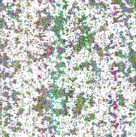
imsegment	Segment binary image to blobs
-src <name>	source name
-cout <name>	class information destination name
-dout <name>	pixel information destination name
-blobindex <boolean>	include blob indexes [false $\vert$ true]
imfloodsegment	Segment gray image to blobs
-src <name>	source name
-cout <name>	class information destination name
-dout <name>	pixel information destination name
-blobindex <boolean>	include blob indexes [false $\vert$ true]
impeaksegment	Segment gray image to blobs
-src <name>	source name
-cout <name>	class information destination name
-dout <name>	pixel information destination name
-blobindex <boolean>	include blob indexes [false $\vert$ true]

These commands are used to segment the image into smaller subregions of more interest. imsegment uses a 4-pixel neighbourhood on the binary image to assess which pixels belong to the same subregion a.k.a. segment, blob, grain. imfloodsegment finds high points in the intensity landscape and fills the hills one by one. impeaksegment finds highest points also but fills all the hills at the same time. All of these methods result in a different type of segmentation. All three methods return a classification and a dataframe with fields x and y for pixel locations. Optionally blob index may be stored in blob field.

imsegment imfloodsegment

impeaksegment

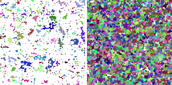
imsegmentcoloring	Color image segments (blobs) with specified color
-src <name>	source name
-dest <name>	destination name
-segdata <name>	segmentation data
-inst <name>	instructions for coloring
imfastsegmentcoloring	Color image segments (blobs) with specified color
-src <name>	source name
-dest <name>	destination name
-segcl <name>	segmentation cldata
-segdata <name>	segmentation data
-inst <name>	instructions for coloring

These commands allow user to alter segment's pixel values to match a spesific color. The -inst dataframe must contain fields blob which identifies which segment is to be colored and color which has the 0-255 intensity value.

Example: In this example segment the image into small blobs and color some of these blobs.

imload -n image -f paper.gif
imfilter -src image -dest image2 -o 0 -s 2
imfindthreshold -src image2 -m percent -p 20 -fout th
imthreshold -src image2 -dest image3 -value ${th}
imsegment -src image2 -cout segcl -dout segdata -blobindex true
len -n segcl -fout len
serie -len ${len} -fout blob
setdata -f color -t int -len ${len} -vals 0=0;
expr -fout color -expr 'color'+IRAND(256);
select inst -f blob color
imsegmentcoloring -src image2 -dest image3 -segdata segdata \
                  -inst inst
im2image -gray image3 -dest oldimage
mkgrp g
bgimg g -img oldimage
show g

Stochastic geometry commands

imtoppoints	Finds top points from an image
-i <name>	source image name
-dout <name>	point field information
-s <size>	turf size (turf has rectangular shape)
[-neq]	deny equal value points inside the mask

This command attempts to find hilltops in the intensity landscape. The resulting dataframe will contain fields x and y for spatial position. Normally points tolerate other points of the same intensity on their turf. Using [-neq] option removes this possibility.

imtoppoints2	Finds top points from an image
-i <name>	source image name
-dout <name>	point field information
-s <size>	turf size (turf has circular shape)
[-neq]	deny equal value points inside the mask

This command is an another way to find hilltops in the intensity landscape. The resulting dataframe will contain fields x and y for spatial position. Normally points tolerate other points of the same intensity on their turf. Using [-neq] option removes this possibility.

imcenterpoints	Find blob center according to indicator function
-i <name>	source image name
-c <name>	class information
-d <name>	pixel information
-dout <name>	point field information
immasspoints	Find blob center according to mass function
-i <name>	source image name
-c <name>	class information
-d <name>	pixel information
-dout <name>	point field information
impeakpoints	Find blob center according to peak indicator function
-i <name>	source image name
-c <name>	class information
-d <name>	pixel information
-dout <name>	point field information

These commands calculate a center for each segment. The resulting dataframe will contain fields x and y for spatial position.

imgundersen	Classify points in a point field according to their location
-i <name>	source image name
-c <name>	class information
-d <name>	pixel information
-dout <name>	point field information
-m <name>	border mode [0=percent $\vert$ 1=pixel]
-v <name>	border width

This command classifies spatial points according to their location into three categories. This classification is placed in a field named frame. Frame value 0 means that the points is to be included into calculations. Value 1 means that point is included in the calculations but is not included in the actual result. Value 2 means that point lies in the forbidden area and is banned from all calculations. For more information, please see page 223 in Stochastic Geometry and its Applications, by Stoyan, Kendall and Mecke.

immarks	Calculate point mark information from blob information
-i <name>	gray image name
-bwi <name>	binary image name
-c <name>	class information
-d <name>	pixel information
-dout <name>	point field information
[-avgvar]	include blob's average and variance information
[-eig]	include blob's principal components and their weights
[-card]	include blob's cardinality
[-border]	include blob's border's cardinality
[-mass]	include blob's mass infomation
[-minmax]	include blob's minimum and maximum intensity information
[-hist]	include blob's grayscale histogram's information
[-rou]	include roundness information
[-rad]	include radii information
[-ecc]	include eccentricity information
[-ste]	include steepness information
[-ori]	include orientation information

This command calculates descriptive features from the segments.

Example: In this example we form a point field based on segmentation information. In order to avoid border effects we use a technique called Gundersen framing. We also count some mark information to describe these points.

imload -n image -f paper.gif
imfilter -src image -dest image2 -o 0 -s 2
imfindthreshold -src image2 -m percent -p 20 -fout th
imthreshold -src image2 -dest image3 -value ${th}
imsegment -src image2 -cout segcl -dout segdata -blobindex true
immasspoints -i image2 -c segcl -d segdata -dout points
imgundersen -i image2 -c segcl -d segdata -dout points -m 1 -v 50
immarks -i image -c segcl -d segdata -dout points \
          -card -border -hist

impointfieldstat	Calculate point field second- and third-order statistics
-i <name>	source image name
-d <name>	point field information
-dout <name>	statistical curves
[-fout <name>]	estimated lambda (average intensity)
-pnts <count>	point count in curves
-radd <count>	r step between points
[-px <position>]	horizontal point position for Lx and gx
[-py <position>]	vertical point position for Lx and gx
[-m <field>]	mark field for mark correlation
[-test <test>]	test for mark correlation [1=area $\vert$ 2=angle in [0,$\pi$] ]
[-mask <mask>]	mask type for third-order statistics [1=rectangle $\vert$ 2=rhombus $\vert$ 3=circle]
[-asize <size>]	mask width for third-order statistics
[-bsize <size>]	mask height for third-order statistics
[-r]	include r-axis
[-K]	include Ripleys K-function
[-L]	include L-function
[-g]	include pair correlation function
[-Lx]	include local L-function
[-gx]	include local pair correlation function
[-k]	include mark correlation function
[-z]	include third-order statistic function
[-ref]	include Poisson functions for reference

This command calculates point field statistics. For more information, please see pages 275-305 in Fractals, Random Shapes and Point Fields, by Stoyan and Stoyan.

Example: In this example we calculate Ripleys K-function of the point field.

impointfieldstat -i image -d points -dout k -pnts 101 \
                 -radd 0.5 -r -K -ref
mkgrp K
select stat -f k.K k.ref_K
fldstat -d stat -dout stat2 -min -max
fldstat -d stat2 -dout stat3 -min -max
len -fout len -n k.r
expr -fout len -expr 'len'-1;
ldgrv K -inx 0 -f k.ref_K -co red -sca abs -min ${stat3.min[0]} \
      -max ${stat3.max[1]}
ldgrv K -inx 0 -f k.K -co black -sca abs -min ${stat3.min[0]} \
      -max ${stat3.max[1]}
saxis K -inx 0 -ax x -sca abs -min ${k.r[0]} \
      -max ${k.r[${len}]} -step 2
saxis K -inx 0 -ax y -sca abs -min ${stat3.min[0]} \
      -max ${stat3.max[1]} -step 2
rm stat
rm stat2
rm stat3
rm len
viewp K -dz -150
show K

Example: In this example we calculate local pair correlation function of the point field.

impointfieldstat -i image2 -d points -dout gx -pnts 101 \
                 -radd 0.5 -r -gx -ref -px 256 -py 256
mkgrp Gx
select stat -f gx.gx gx.ref_gx
fldstat -d stat -dout stat2 -min -max
fldstat -d stat2 -dout stat3 -min -max
len -fout len -n gx.r
expr -fout len -expr 'len'-1;
ldgrv Gx -inx 0 -f gx.ref_gx -co red -sca abs \
      -min ${stat3.min[0]} -max ${stat3.max[1]}
ldgrv Gx -inx 0 -f gx.gx -co black -sca abs \
      -min ${stat3.min[0]} -max ${stat3.max[1]}
saxis Gx -inx 0 -ax x -sca abs -min ${gx.r[0]} \
          -max ${gx.r[${len}]} -step 2
saxis Gx -inx 0 -ax y -sca abs -min ${stat3.min[0]} \
          -max ${stat3.max[1]} -step 2
rm stat
rm stat2
rm stat3
rm len
viewp Gx -dz -150
show Gx

Example: In this example we calculate mark correlation function of the point field.

impointfieldstat -i image2 -d points -dout markcorrelation \
                 -pnts 101 -radd 0.5 -r -k -ref -m are -test 1
mkgrp MarkCorrelation
select stat -f markcorrelation.k_are markcorrelation.ref_k_are
fldstat -d stat -dout stat2 -min -max
fldstat -d stat2 -dout stat3 -min -max
len -fout len -n markcorrelation.r
expr -fout len -expr 'len'-1;
ldgrv MarkCorrelation -inx 0 -f markcorrelation.ref_k_are \
      -co red -sca abs -min ${stat3.min[0]} -max ${stat3.max[1]}
ldgrv MarkCorrelation -inx 0 -f markcorrelation.k_are -co black \
      -sca abs -min ${stat3.min[0]} -max ${stat3.max[1]}
saxis MarkCorrelation -inx 0 -ax x -sca abs \
      -min ${markcorrelation.r[0]} \
      -max ${markcorrelation.r[${len}]} -step 2
saxis MarkCorrelation -inx 0 -ax y -sca abs \
          -min ${stat3.min[0]} -max ${stat3.max[1]} -step 2
rm stat
rm stat2
rm stat3
rm len
viewp MarkCorrelation -dz -150
show MarkCorrelation

Example: In this example we calculate the third-order statistic of the point field.

impointfieldstat -i image2 -d points -dout z -pnts 101 -radd 0.5 \
                 -r -z -ref -mask 1 -asize 0.5 -bsize 0.25
mkgrp Z
select stat -f z.z z.ref_z
fldstat -d stat -dout stat2 -min -max
fldstat -d stat2 -dout stat3 -min -max
len -fout len -n z.r
expr -fout len -expr 'len'-1;
ldgrv Z -inx 0 -f z.ref_z -co red -sca abs -min ${stat3.min[0]} \
          -max ${stat3.max[1]}
ldgrv Z -inx 0 -f z.z -co black -sca abs -min ${stat3.min[0]} \
          -max ${stat3.max[1]}
saxis Z -inx 0 -ax x -sca abs -min ${z.r[0]} \
          -max ${z.r[${len}]} -step 2
saxis Z -inx 0 -ax y -sca abs -min ${stat3.min[0]} \
          -max ${stat3.max[1]} -step 2
rm stat
rm stat2
rm stat3
rm len
viewp Z -dz -150
show Z

imnearestneighbour	Calculate contact information in a point field
-d <name>	point field information
-dout <name>	point field information
-k <count>	count values for 1-k neighbours
[-index]	include indexes to nearest neigbours
[-angle]	include angles to nearest neigbours
[-cumangle]	include cumulative angles to nearest neigbours
[-contangle]	include continuing angle to nearest neigbours
[-dist]	include distances to nearest neigbours
[-cumdist]	include cumulative distances to nearest neigbours
[-contdist]	include continuing distances to nearest neigbours

This command calculates nearest neighbour information.

Example: In this example we inspect contact distributions in the point field.

...
imnearestneighbour -d points -dout points -k 3 -dist -angle

imrandpoints	Generate a random point field with uniform distribution
-dout <name>	point field information
-pnts <points>	points in the point field
-w <width>	width of the point field
-h <height>	height of the point field

This command is used to generate a random point process for testing purposes. Points are generated from a 2D uniform distribution.

imkernel2d	Kernel estimate a 2D process
-p <name>	point process dataframe
-t <name>	test process dataframe
-dout <name>	estimated angles, distances, and weights
-k <value>	kernel type [1=box $\vert$ 2=pyramid $\vert$ 3=cylinder $\vert$ 4=cone $\vert$ 5=half sphere $\vert$ 6=gaussian]
-V <value>	kernel size
-c <value>	cut distance (ignore points further than this)
imknn2d	KNN estimate a 2D process
-p <name>	point process dataframe
-t <name>	test process dataframe
-dout <name>	estimated angles, distances, and weights
-k <value>	kernel type [1=box $\vert$ 2=pyramid $\vert$ 3=cylinder $\vert$ 4=cone $\vert$ 5=half sphere $\vert$ 6=gaussian]
-K <value>	kernel point size
-c <value>	cut distance (ignore points further than this)
imkernel1d	Kernel estimate a weighted dataset
-v <name>	field of data
-p <name>	field of priories
-dout <name>	estimated distribution
-pins <value>	number of pins
-a <value>	axis minimum
-b <value>	axis maximum
-k <value>	kernel type [1=box $\vert$ 2=triangle $\vert$ 3=half circle $\vert$ 4=gaussian]
-V <value>	kernel size
-c <value>	cut distance (ignore points further than this)
imknn1d	KNN estimate a weighted dataset
-v <name>	field of data
-p <name>	field of priories
-dout <name>	estimated distribution
-pins <value>	number of pins
-a <value>	axis minimum
-b <value>	axis maximum
-k <value>	kernel type [1=box $\vert$ 2=triangle $\vert$ 3=half circle $\vert$ 4=gaussian]
-K <value>	kernel point size
-c <value>	cut distance (ignore points further than this)

These commands are used to estimate distributions of the point processes. 2D methods take a point field and return information on all available point pairs. 1D methods are used to generate the distribution based on weighted point pairs.

Example: In this example we use two estimators to estimate the angle and distance distributions from the point process.

...
imrandpoints -dout test -pnts 1000 -w 512 -h 512

imkernel2d -p points -t test -dout distdata1 -V 50
expr -fout distdata1.weight -expr 'distdata1.weight' * 1000000.0;
imkernel1d -v distdata1.angle -p distdata1.weight \
           -dout angle1 -V 0.1
imkernel1d -v distdata1.distance -p distdata1.weight \
           -dout distance1 -V 1 -a 0 -b 100
mkgrp Angle1
ldgrv Angle1 -f angle1.value
show Angle1
mkgrp Distance1
ldgrv Distance1 -f distance1.value
show Distance1

imknn2d -p points -t test -dout distdata2 -K 10
expr -fout distdata2.weight -expr 'distdata2.weight' * 1000000.0;
imkernel1d -v distdata2.angle -p distdata2.weight \
           -dout angle2 -V 0.1
imkernel1d -v distdata2.distance -p distdata2.weight \
           -dout distance2 -V 1 -a 0 -b 100
mkgrp Angle2
ldgrv Angle2 -f angle2.value
show Angle2
mkgrp Distance2
ldgrv Distance2 -f distance2.value
show Distance2

Simulation commands

imsimspectralmethod	Simulate an image
-iout <name>	image name
-w <value>	image width
-h <value>	image height
-m <method>	image simulation method [ circular $\vert$ spherical $\vert$ exponential $\vert$ gaussian $\vert$ kbessel ]
-a <value>	image simulation scaling

This command simulates an image using the spectral method. For more information, please see pages 191-192 in Geostatistical Simulation by C. Lantuejoul.

Graph commands

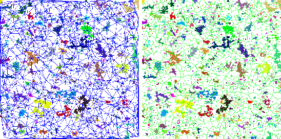
imvoronoi	Generates Delaunay/Voronoi diagrams (based on Steven Fortune's algorithm)
-d <name>	vertex information
-dout <name>	edge information
[-dout2 <name>]	point field information (needed for Voronoi diagrams)
[-sites <value>]	number of sites
[-xmin <value>]	minimum x value
[-xmax <value>]	maximum x value
[-ymin <value>]	minimum y value
[-ymax <value>]	maximum x value
[-d]	echo debug information
[-s]	data is sorted
[-t]	generate Delaunay diagram (default: Voronoi diagram)
[-p]	plot information

This command is used to build Delaunay and Voronoi triangulations based on x and y fields in the vertex dataframe. In Delaunay case, a dataframe with fields v1 and v2 is generated. Field v1 is the index of starting vertex and v2 is the index of the ending vertex. In Voronoi case a dataframe containing new vertex information is also generated.

imnetangleslenghts	Count edge angles and lenghts
-v <name>	vertex information
-e <name>	edge information

This command is used to calculate angle and distance information from a graph.

imbuildnet	Build a line graph suitable for vecfld command
-v <name>	vertex information
-e <name>	edge information
-dout <name>	line graph
-w <width>	image width
-h <height>	image height

This command is used to quickly build a linegraph for vecfld.

Example: In this example we use a point field to create Delaunay and Voronoi diagrams.

...
# create delaunay graph
imvoronoi -d points -dout delaunay -t
imnetangleslenghts -v points -e delaunay
imbuildnet -v points -e delaunay -dout delaunaynet -w 512 -h 512
# create a voronoi graph
imvoronoi -d points -dout voronoi -dout2 voronoipoints
imnetangleslenghts -v voronoipoints -e voronoi
imbuildnet -v points -e delaunay -dout delaunaynet -w 512 -h 512
# show graphs over the bitmap
mkgrp g
bgimg g -img oldimage
vecfld g -n delaunay -d delaunaynet -co blue
vecfld g -n voronoi -d voronoinet -co green
show g

Delaunay diagram Voronoi diagram

Fractal commands

imfractal	Count fractal features from an image
-i <name>	source image name
-dout <name>	feature information
[-curve <name>]	curve points where features are extracted
-xadd <size>	horizontal step
-yadd <size>	vertical step
-xsize <size>	horizontal max.size
-ysize <size>	vertical max. size

This command calculates a few fractal features from a gray image.

Example: In this example we calculate fractal features from an image.

imload -n image -f paper.gif
imfractal -i image -dout features -curve curve -xadd 512 -yadd 512 \
          -xsize 512 -ysize 512 -pnts 7
mkgrp g
axis g -ax x -f curve.x
datplc g -n plt -ax x -f curve.x -co blue
axis g -ax y -f curve.y
datplc g -n plt -ax y -f curve.y -co blue
viewp g -dz -111
show g