Next: File I/O Up: User's reference Previous: Revised image processing commands Contents

Subsections

Graphics

The graphical state of created windows is stored as structures, which can be handled through the commands documented in this section. The operations change the state of the specified graphic structure. The graphical subsystem contains two representation levels. The higher level defines graphical objects by their meanings such as bar, data scatterplot and so on. A lower level representation is generated from the higher level objects when a window needs redrawing. The lower level contains only really primitive graphical elements (line, circle, polygon, text). Therefore, the lower level representation can easily be displayed using any graphical user interface with a straightforward technical implementation.

Creating and initializing graphic structures

The following commands create and initialize a graphic structure. The graphic structure consists of several so-called subgraphs. The subgraphs may have their own graphical elements, but most of the graphical commands change the properties of all subgraphs within the same graphical structure.

There are three possible ways to create a graphic structure:

SOM: To visualize a specific neural network structure (TS-SOM), it can be specified as a parameter. In this case each neuron will have its own subgraph.
Data: Graphics structure can also be created for a data frame, in which case each subgraph will correspond to one data record.
Manual: If no source data or SOM is specified, subgraphs must be created with addsg (see section 8.1.2). If data records are to be displayed in subgraphs, then a source data frame must be connected to a graphic structure with setgdat (see section 8.1.1) and a data record for one subgraph is selected with setsg (Sect. 8.1.2).

In addition, a classified data frame can be connected to a graphic structure, but its use depends on chosen operations.

Creating a graphic structure and connecting a frame to it

mkgrp Create a new graphic structure

<graphic> name for the graphic structure

[{-s <som> | a TS-SOM structure

-d <data>}] a data frame

setgdat Connect a data frame to graphics

<graphic> name of the graphic structure

-d <data> a data frame

setgcld Connect a classified data frame to graphics

<graphic> name of the graphic structure

-c <cldata> a classified data frame

Operation mkgrp creates a basic graphic structure. The graphic structure contains several subgraphs, which can be created manually with addsg, or according to a TS-SOM structure or a data frame.

The commands setgdat and setgcld connect a data frame and a classified data frame, respectively, to a graphic structure. Some graphical operations are able to use these as default parameters for <data> and <cldata>. In the case of TS-SOMs, a graphic structure can visualize any variables in neurons, and the classified data needs to be a SOM classification.

Example (ex7.1): The first command sequence creates a TS-SOM and a classified data and computes class statistics for the neurons.

...
NDA> somtr -d boston -sout som1 -l 5
...
NDA> somcl -d boston -s som1 -cout cld1
NDA> clstat -d boston -c cld1 -dout clsta -avg -min -max
...

Then the graphic structure grp1 is created based on som1. Both the data frame containing statistics and classified data are connected to the graphic structure.

...
NDA> mkgrp grp1 -s som1
NDA> setgdat grp1 -d clsta
NDA> setgcld grp1 -c cld1

Example (ex7.2): In this example, a graphic structure is created for a data frame, in which case each data record in the frame will have its own subgraph.

NDA> load boston.dat
NDA> selrec -d boston -dout highCrim -expr 'boston.crim' > 35;
NDA> mkgrp grp1 -d highCrim
...

Managing subgraphs

addsg Create a new subgraph to a graphic structure

<graphic> name of the graphic structure

setsg Connect a data record to a subgraph

<graphic> name of the graphic structure

-inx <index> index of the subgraph

-rec <recinx> index of the data record

rmsg Remove the specified subgraph

<graphic> name of the graphic structure

-inx <index> index of the subgraph

If the specified graphic structure is not based on a data frame or a TS-SOM structure, subgraphs must be created manually. The command addsg creates a new subgraph and returns the index of the created subgraph. The command setsg connects data records to subgraphs. The command rmsg removes the specified subgraph.

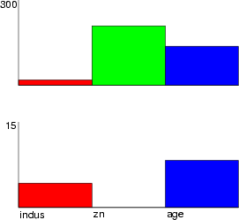
Example (ex7.3): The following commands create two subgraphs and connects them to data records. The data record 15 is connected to the first subgraph and data record 300 to the second subgraph.

To illustrate results, two bars are created from the fields of Boston data. The last command writes the resulting graph to a PostScript file.

NDA> load boston.dat
NDA> mkgrp grp1
NDA> addsg grp1
0
NDA> setsg grp1 -inx 0 -rec 15
NDA> addsg grp1
1
NDA> setsg grp1 -inx 1 -rec 300
NDA> bar grp1 -f boston.crim -co red
NDA> bar grp1 -f boston.zn -co green
NDA> wrps -n grp1 -o koe.ps -w 500 -h 500

$\begin{figure}\centerline{\hbox{ \psfig{figure=lbars.ps,width=6cm} }} \end{figure}$

Setting a structure over subgraphs

The following operations change properties of all subgraphs of the specified graphic structure. These operations need more information about the structure, how the subgraphs are connected. A TS-SOM is a good basis for visualization, but these operations can also use other data structures, such as classified data frames.

Setting the visualized layer

layer Set the layer of TS-SOM

<graphic> name of the graphic structure

-l <layer> index of the layer

[-min <min>] starting layer

This command sets the layer of TS-SOM to be displayed. Also several layers can be displayed simultaneously. The starting layer <min> defines the first layer, while the last is defined by <layer>. To display only one layer, <min> can be omitted. The starting layer can be kept the same as previously by specifying -1 as <min>.

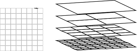
Example (ex7.4): The first example demonstrates the basic setting of the visualized layer. You can see the result in the left-hand side figure below.

...
NDA> mkgrp grp1 -s som1
NDA> layer grp1 -l 3

Example (ex7.5): The second example shows how several layers of TS-SOM can be displayed simultaneously. In this case the layer indexes of TS-SOM must be first stored into a field using somlayer (see section 5.1.4), and the locations of the neurons are set according to the values of this somlayer field. The layers 0-3 are displayed.

...
NDA> somtr -d predata -sout som1 -l 4
...
NDA> somlayer -s som1 -f somlayer
...
NDA> mkgrp grp1 -s som1
NDA> axis grp1 -ax z -f somlayer -sca abs -min 0 -max 5
NDA> nplc grp1 -ax z -f somlayer
NDA> layer grp1 -l 3 -min 0
NDA> viewp grp1 -dz 150 -xy -100 -yz 85
NDA> show grp1

$\begin{figure}\centerline{\hbox{ \psfig{figure=basicsom.ps,width=4cm} \psfig{figure=multilayer.ps,width=6cm} }} \end{figure}$

Setting the topology and child links of TS-SOM

topo Show/hide the topology of TS-SOM

<graphic> name of the graphic structure

-on | -off topology on/off

[-c <cldata>] classified data for links

[-all] show all the links

sons Show/hide child links of the TS-SOM

<graphic> name of the graphic structure

-on | -off child links on/off

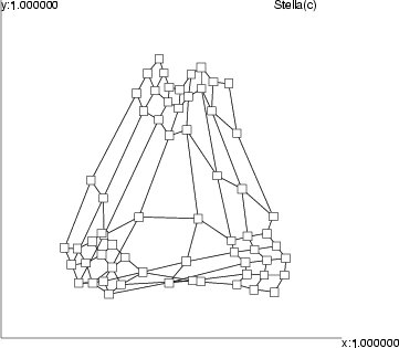
The first operation switches the topology of the network on or off, the second performs the same for child links. If a classified data has been specified, then the topology links are read from it. The classified data must include a class for each data record (neuron), when the links are specified as indexes (see the figure below). If the last flag -all is given, then the links are visible independently of the visibility of the subgraphs. In the example 8.3.6, this flag is not given, and therefore, only those links that have both subgraphs visible are displayed.

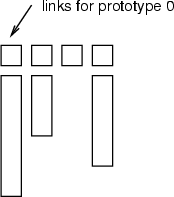
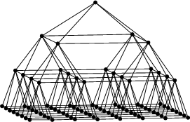
$\begin{figure}\centerline{\hbox{ \psfig{figure=topolinks.ps,width=4cm} }} \end{figure}$

Example (ex7.6): This example shows, how several layers and links between them can be displayed.

...
NDA> somtr -d predata -sout som1 -l 4
...
NDA> somlayer -s som1 -f somlayer
...
NDA> mkgrp grp1 -s som1
NDA> topo grp1 -on
NDA> sons grp1 -on
NDA> layer grp1 -l 3 -min 0
NDA> axis grp1 -ax z -f somlayer -sca abs -min 0 -max 5
NDA> nplc grp1 -ax z -f somlayer
NDA> viewp grp1 -dz 150 -xy -100 -yz 85
# Other settings for neurons, network, etc.
...

$\begin{figure}\centerline{\hbox{ \psfig{figure=sonlinks.ps,width=6cm} }} \end{figure}$

Creating trajectories

traj Create or set a trajectory

<graphic> name of the graphic structure

-n <name> name for the trajectory

-min <min> starting index of data

-max <max> ending index of data

-co <color> color for the trajectory

[-step <step>] step between the labels

[-f <field>] field for labelling. If omitted, indexes are used as labels

[-c <cldata>] another classified data

[-d <ddata>] distance data, which describes the distances between data records and their BMU neurons

traj <graphic> -n <name> -rm Remove trajectory <name>

This operation creates a trajectory onto a TS-SOM layer. Data records (indexes from <min> to <max>) are placed to neurons according to the SOM classification. If a classified data has been connected to a graphic structure with setgcld (see section 8.1.1), it defines the mapping between neurons and data records. However, one can override this by specifying a classified data with flag -c. The default way to locate a trajectory is to set trajectory points in the centroid of the subgraphs. You can adjust the location of trajectory points by specifying a distance data <ddata>. This distance data can be calculated with somproj (see section 5.1.9 and the second example).

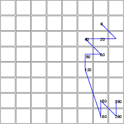
Example (ex7.7): The following command sequence creates a graphic structure called grp1 and connects a classified data to it. Then, it creates a trajectory, which is labelled with data record indexes, which is shown for every 20th data record. Note that the trajectory depends on the layer of the TS-SOM, and it will be updated after setting the current layer.

...
NDA> mkgrp grp1 -s som1
NDA> setgcld grp1 grp1 -c cld1
NDA> layer grp1 -l 3
NDA> traj grp1 -n tr1 -co blue -min 0 -max 300 -step 20

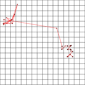
$\begin{figure}\centerline{\hbox{ \psfig{figure=traj.ps,width=5.5cm} }} \end{figure}$

Example (ex7.8): The previous example fixed the trajectory lines to the centroids of the neurons. In this example, we compute a distance data, which describes the distances between data records and their BMU neurons. These distances are used to move the endpoints of trajectory lines from the centroids of the neurons.

Also the classified data alone can be used to map trajectories from distinct data sets to the same SOM. Thus, the projection data (here dmat) is not necessary for this command.

NDA> somproj -s som1 -w som1_W -d predata -c c1 -dout dmat
NDA> mkgrp grp1 -s som1
NDA> setgcld grp1 grp1 -c 1
NDA> layer grp1 -l 3
NDA> traj grp1 -n tr1 -co red -min 0 -max 300 -step 20 -c c1
      -d dmat

$\begin{figure}\centerline{\hbox{ \psfig{figure=trajdis.ps,width=6cm} }} \end{figure}$

Connecting neurons

nconn Connect neurons through external information

<graphic> name of the graphic structure

-n <name> name for the connector

-c <cldata> link information

-min <min> lower boundary for links

-max <max> upper boundary for links

[-co <color>] color for the connector

[-nolab] if the lines should not be labelled with proportions

nconn <graphic> -n <name> -rm Remove connector <name>

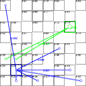
This operation connects neurons according to information represented by a classified data. For each neuron, it contains a class, which contains the links from this particular neuron to other neurons. The links are displayed as lines. The widths of these lines indicate the proportions of links between these two neurons compared to the whole set of links.

Example: As a simple illustration, two neurons have been linked to other neurons. Without describing the procedure in more detail, the following figure gives an idea of possible visual presentations.

$\begin{figure}\centerline{\hbox{ \psfig{figure=nconn.ps,width=8cm} }} \end{figure}$

Creating contours

cntr Set a contour

<graphic> name of the graphic structure

-n <name> name of the contour

-f <field> field to be used for neurons

-v <value> value for the contour (elevation)

[-co <color>] color for the contour

[-t <type>] how the contour is drawn

cntr <graphic> -n <name> -rm Remove contour <name>

The operation creates contour lines onto a TS-SOM layer. The contour line is placed based on the values of <field> in neurons and the specified value <value>. The field values in neurons are compared to the specified value, and the line goes through points, in which the interpolated field value between neighboring neurons equals to <value>.

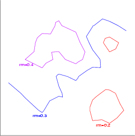
Example (ex7.9): This example shows, how contours can be created. In this case a TS-SOM has been trained with Boston data. Three contours are created to describe the changes of weight rm_w with values 0.2, 0.3 and 0.4 on layer 3.

...
NDA> mkgrp grp1 -s s1
NDA> layer grp1 -l 3
NDA> cntr grp1 -n rm=0.2 -co red -f s1_W.rm_w -v 0.2
NDA> cntr grp1 -n rm=0.3 -co blue -f s1_W.rm_w -v 0.3
NDA> cntr grp1 -n rm=0.4 -co magenta -f s1_W.rm_w -v 0.4

$\begin{figure}\centerline{\hbox{ \psfig{figure=cntr.ps,width=6cm} }} \end{figure}$

The U-matrix presentation

umat Set a U-matrix to be used while visualizing a graphic structure

<graphic> name of the graphic structure

-umat <umat> name of the U-matrix data to be used

umat <graphic> -rm Clear the U-matrix presentation

This command sets a U-matrix to be used while visualizing the specified graphic structure. The distances between neurons are illustrated as distances between the rectangles in a graphical presentation. See the umat command (section 5.1.7) for information about how U-matrices are calculated.

Example (ex7.10): Three weights, rm_w, zn_w and age_w, are selected to be the basis of distance computing. Then a U-matrix is computed and selected into graphic structure grp1.

...
NDA> somtr -d boston -sout s1 -l 5
...
NDA> mkgrp grp1 -s s1
...
NDA> select umatflds -f s1_W.rm_w s1_W.zn_w s1_W.age_w
NDA> calcumat -s s1 -d umatflds -umat umat1
NDA> umat grp1 -umat umat1

$\begin{figure}\centerline{\hbox{ \psfig{figure=umat.ps,width=5cm} }} \end{figure}$

Axis for each dimension - x, y and z

axis Set an axis

<graphic> name of the graphic structure

-ax <axis> name of the axis: x, y or z

[-sca <scaling>] scaling function

[-f <field>] field for computing the scale

[-min <min>] minimum value

[-max <max>] maximum value

[-step <scales>] the number of scale labels

axis <graphic> -ax <axis> -rm Remove axis <axis>

The graphic structure has one global coordinate system (x, y and z axes). Command axis computes the scale for the specified axis (using the minimum and maximum values). The normal scaling function (see section 8.5) is available, but note, that this command does not locate any data points or neurons in a neural network related to an axis.

Parameter -step defines the number of ranges for displaying the labels of the scale for the axis. The whole range of the axis (from <min> to <max>) is divided into uniform parts.

See the examples of datplc (section 8.2.8) and nplc (section 8.3.1).

3D scatterplotting

datplc Scatter the values of a data vector to one axis

<graphic> name of the graphic structure

-n <setname> name of the scatterplot

-ax <axis> name of the axis: x, y or z

-f <field> data field to be scattered

[-co <color>] color for data points

[-volume <vol_size>] size

[-shape <shape>] shape

[-shape_data <char>] shape data (for character shape)

datplc <graphic> -n <name> -rm Remove scatterplot <name>

To scatter data points, datplc computes the locations of <field> values related to the specified axis (set with axis, see section 8.2.7). Several data sets identified with <name> can be displayed using different colors. <vol_size> is the size of individual record in dataplot (0.005 is default). Parameter <shape> can be dot (2D - default), pyramid (3D), cross (3D), cube (3D), or character (2D). With shape character one must also define parameter <char>, which defines the character which is to be used for drawing the dataset.

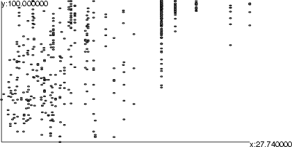
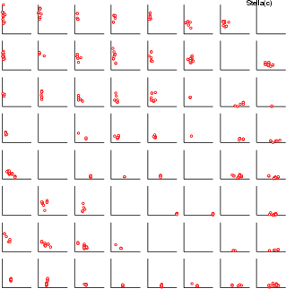
Example 1 (ex7.11): The x axis is set according to the field indus. Since the parameter <scaling> is omitted, the minimum and maximum values of the axis are located from the specified field. In other words, the default scaling function is data. The same procedure is performed for the y axis.

NDA> load boston.dat
NDA> mkgrp grp1
NDA> axis grp1 -ax x -f boston.indus
NDA> datplc grp1 -n boston -ax x -f boston.indus
NDA> axis grp1 -ax y -f boston.age
NDA> datplc grp1 -n boston -ax y -f boston.age
NDA> show grp1

Example 2: The following commands demonstrate the use of switches -shape and -volume.

NDA> mkgrp grp2
NDA> select flds -f boston.indus boston.flds
NDA> datplc grp2 -n flds -ax x -f flds.indus
NDA> datplc grp2 -n flds -ax y -f flds.dis -co green \
     -volume 0.008 -shape cross
NDA> datplc grp2 -n flds_text -ax x -f flds.indus
NDA> datplc grp2 -n flds_text -ax y -f flds.dis -co magenta \
     -shape character -shape_data b
NDA> show grp2

This image shows the result of the first example above.

$\begin{figure}\centerline{\hbox{ \psfig{figure=datplc.ps,width=11cm} }} \end{figure}$

Setting the graphical contents of subgraphs

These operations define the outlook of subgraphs (neurons). Several features, such as locations, colors, sizes, shapes and visibility, can be altered.

Setting the locations of neurons in 3D

nplc Set the places of neurons related to an axis

<graphic> name of the graphic structure

-ax <axis> name of the axis: x, y or z

-f <field> data field for the locations

nplc <graphic> -ax <axis> -rm Set the neuron locations for one specified axis to 0.0

This operation sets the locations of neurons related to the x, y or z axis in three-dimensional space. Before using this command, the scale of the axis should be computed with axis (see section 8.2.7). The reserved field names som_x, som_y and som_z set the locations of neurons to the normal grid of the SOM.

Example (ex7.12): The following commands set the scales of the axes x and y to the absolute range [0,1]. Then, the locations of neurons are set according to two weights x_w and y_w. At the end, the visible layer is set to 3.

...
NDA> somtr -d gauss.dat -sout som1 -l 5
...
NDA> mkgrp grp1 -s som1
NDA> nsize grp1 -v 0.2
NDA> topo grp1 -on
NDA> axis grp1 -ax x -sca abs -min 0.0 -max 1.0
NDA> axis grp1 -ax y -sca abs -min 0.0 -max 1.0
NDA> nplc grp1 -ax x -f som1_W.x_w
NDA> nplc grp1 -ax y -f som1_W.y_w
NDA> layer grp1 -l 3
...

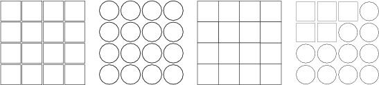
$\begin{figure}\centerline{\hbox{ \psfig{figure=nplc.ps,width=8cm} }} \end{figure}$

Setting the shape of the neurons

nshape Set the shape of the neurons

<graphic> name of the graphic structure

<shape> Chosen shape: rectangle | polygon | circle

[-expr <expr>;] a boolean expression

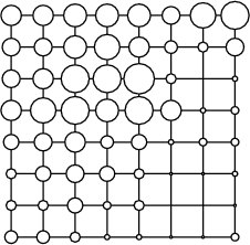
This operation selects the shape of the subgraphs for neurons. polygon is different from rectangle in the aspect that neurons are always connected to each other and only the center of each neuron is located at the chosen z axis location. Borders of polygons attempt to interpolate the z values of neighbor neurons. If the boolean expression is given, then the shape is changed only in those neurons in which the truth value is true.

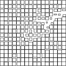
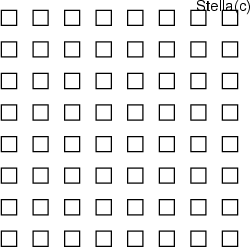
Example (ex7.37): An organized TS-SOM is displayed with three types of neurons. Choice rectangle is the default value. The last command sets the shape conditionally according to the rule.

...
NDA> mkgrp grp1 -s s1
NDA> layer grp1 -l 2
NDA> nshape grp1 rectangle
NDA> nshape grp1 circle
NDA> nshape grp1 polygon
NDA> nshape grp1 circle -expr 'sta.crim_avg' < 1;
...

$\begin{figure}\centerline{\hbox{ \psfig{figure=rect.ps,width=2.7cm} \hspace{0.2c... ...th=2.7cm} \hspace{0.2cm} \psfig{figure=shapeexpr.ps,width=2.7cm} }} \end{figure}$

Setting the size of neurons

nsize Set the size of neurons

<graphic> name of the graphic structure

-v <value> size for the neurons (usually relative to the SOM grid)

[-abs] <value> is to be used as an absolute value; otherwise it is relative to the SOM grid (default)

The sizes of the subgraphs can be set in two ways. The first possibility is to change the size of all (rectangular or circular) neurons using nsize. The parameter <value> usually means: relative to the basic size, which is computed based on the grid of the SOM. The second possibility is to specify the diameters of circular neurons using ndiam (described in section 8.3.4).

Example (ex7.13): The size of neurons is set to 0.5, which means that it is half of the distance between two neighboring neuron locations in the SOM grid.

...
NDA> mkgrp grp1 -s s1
NDA> layer grp1 -l 3
NDA> nsize grp1 -v 0.5

$\begin{figure}\centerline{\hbox{ \psfig{figure=nsize.ps,width=7cm} }} \end{figure}$

Setting the proportional diameters of circular neurons

ndiam Set the diameter of circular neurons

<graphic> name of the graphic structure

-f <field> name of the field

[-sca <scaling>] scaling function

[-min <min>] minimum value

[-max <max>] maximum value

ndiam <graphic> -rm Set relative diameters to 1.0

This operation sets the proportional diameters of the circles computed using the values of a specified data field. This command only affects the size of circular neurons.

Example (ex7.14): The diameter is set to describe the weight rm_w. Also the topology of the SOM is switched on. The diameter is scaled in such a way that the minimum value in the current layer corresponds to the relative diameter value 0 and the maximum value to 1.

...
NDA> mkgrp grp1 -s s1
NDA> layer grp1 -l 3
NDA> topo grp1 -on
NDA> ndiam grp1 -f s1_W.rm_w -sca som

$\begin{figure}\centerline{\hbox{ \psfig{figure=ndiam.ps,width=5cm} }} \end{figure}$

Setting the colors or gray levels of neurons

ncolor Set the color of neurons

<graphic> name of the graphic structure

-fg <fgcolor> foreground color

-bg <bgcolor> background color

[-expr <expr>;] a boolean expression

ngray Set the gray level for the background of the neurons

<graphic> name of the graphic structure

-f <field> source field for evaluating gray levels

[-sca <scaling>] scaling function, default=SOM

[-min <min>] minimum value

[-max <max>] maximum value

[-rgb] use the pseudo colors instead of gray levels

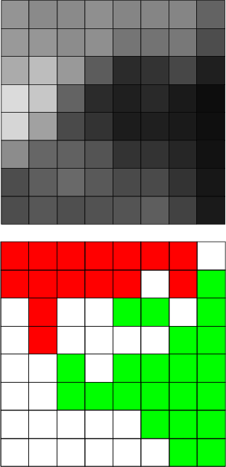
The background color of the neurons can be set in two different ways. The first command ncolor is also able to set the foreground color. If the last parameter, the boolean expression, is given, then the color settings are changed only in neurons for which the expression gives the truth value true.

The second command sets the gray level of the background of the neurons based on the values of a specified variable <field>. The functionality of the last parameter -rgb depends on the used computing environment, but it should produce a pseudo color map having colors from blue to green and further to red.

Example (ex7.15): The following commands set the gray level of the background of the neurons based on weight indus_w. The latter two commands set conditionally background of the neurons according to the given rules.

...
NDA> somtr -d boston -sout s1 -l 5
...
NDA> mkgrp grp1 -s s1
NDA> layer grp1 -l 3
NDA> ngray grp1 -f s1_W.indus_w
...
NDA> ncolor grp1 -bg red -expr 'statdata.crim_avg' > 1;
NDA> ncolor grp1 -bg green -expr 'statdata.zn_avg' > 3;
...

$\begin{figure}\centerline{\hbox{\vbox{ \psfig{figure=ngray.ps,width=7cm} \vspace{0.5cm} \psfig{figure=ncolor.ps,width=7cm} } }} \end{figure}$

The visibility of the neurons

nvsbl Set the visibility of neurons

<graphic> name of the graphic structure

-expr <expr>; boolean expression to be evaluated using the variables in the neurons

[-v] verbose evaluation

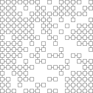
This command evaluates the given expression for each neuron and sets visible those neurons, which return a TRUE value. Typically the fields in the expression should be variables of the neurons.

Example (ex7.16): The following commands hide those neurons, which do not represent any data records.

...
NDA> somtr -d predata -sout s1 -l 5
...
NDA> somcl -d predata -s s1 -cout cld1
NDA> clstat -d boston -c cld1 -dout statdata -hits
...
NDA> mkgrp grp1 -s s1
NDA> setgdat grp1 -d statdata
...
NDA> nvsbl grp1 -expr 'statdata.hits' > 0; -v
{{10} > {0}} => TRUE}
{{0} > {0}} => FALSE}
...

$\begin{figure}\centerline{\hbox{ \psfig{figure=nvsbl.ps,width=7cm} }} \end{figure}$

Graphical presentations inside subgraphs

These commands are meant for setting graphical properties of subgraphs. Each subgraph is connected to some data record being displayed. For instance, each neuron refers to a data record which contains the variable values for that neuron. If a graphic structure has several subgraphs, the commands alter the visualization of all these subgraphs.

Axes in subgraphs

saxis Show an axis in the subgraphs

<graphic> name of the graphic structure

-ax <axis> name of the axis: x, y or z

[-inx <index>] index of the subgraph

[-sca <scaling>] scaling function, default=DATA

[-f <field>] source field

[-min <min>] minimum value

[-max <max>] maximum value

[-step <lab-step>] number of labels

saxis <graphic> -ax <axis> [-inx <index>] -rm

Remove the axis definition

This command sets an axis for the subgraphs. These axes are only used to provide information about the ranges of the axes. They do not define the places of any objects. In addition, several operations, such as bars, skip over this definition and they place the bar objects in the default range [0,1]. If the parameter <index> has been specified, then the axis definition is meant for this single subgraph. Otherwise the definition is used for all available subgraphs. For an example, see section 8.4.2.

Plotting data in subgraphs

ndatplc Set a data field for an axis to enable data plotting

<graphic> name of the graphic structure

-n <name> name of the data to be plotted

-ax <axis> name of the axis: x, y or z

-f <field> source field

-c <cldata> a classified data

[-co <color>] the color of the data points

ndatplc <graphic> -n <name> -rm

Remove a data set

This command maps a given data field to the axes of the subgraphs in a way that <cldata> determines, which data records are mapped to which neurons. Before using this command, the definition of the axes should be set with saxis.

Example (ex7.33): In the following example, the correlation of two fields inside neurons is visualized through data plotting.

...
# Results from a normal SOM analysis: som, cld
# Original data in frame boston
NDA> mkgrp grp1 -s som
NDA> saxis grp1 -ax x -sca data -min boston.nox -max boston.nox
NDA> ndatplc grp1 -n set1 -ax x -f boston.nox -c cld -co red
NDA> saxis grp1 -ax y -sca data -min boston.dis -max boston.dis
NDA> ndatplc grp1 -n set1 -ax y -f boston.dis -c cld -co red

$\begin{figure}\centerline{\hbox{ \psfig{figure=ndatplc.ps,width=9cm} }} \end{figure}$

Bars in subgraphs

bar Create or alter a bar

<graphic> name of the graphic structure

[-inx <index>] bar index

-f <field> source data field

[-sca <scaling>] scaling function, default=SOM

[-min <min>] minimum value

[-max <max>] maximum value

[-co <color>] color for the bar

[-expr <bool-expr>] boolean expression

bar <graphic> -f <field> -rm Remove a bar

This command creates bars to all subgraphs in a graphic structure. The <index> defines the place of this bar related to other specified bars. The scaling parameters are documented in a greater detail in section 8.5. The boolean expression can be used to show bars only for a part of the subgraphs. Only if the value of the expression is TRUE for a data record corresponding to a subgraph, a bar is created. More information about the evaluation of expressions can be found in section 4.4.1.

This operation creates the high level representation for a bar. In addition, the user can select the final appearance of the bars by selecting different modes for bar display (see commands en and dis in section 8.10).

Example (ex7.17): The following commands create two bars for displaying the average values of crim_avg and zn_avg in a SOM-oriented graphic structure.

...
NDA> clstat -c cld1 -d boston -dout stadata -all
...
NDA> mkgrp grp1 -s som
NDA> setgdat grp1 -d stadata
NDA> layer grp1 -l 3
NDA> bar grp1 -f stadata.crim_avg -co red
NDA> bar grp1 -f stadata.zn_avg -co green
NDA> en grp1 bar barflat
NDA> dis grp1 barflat barlab saxis
...

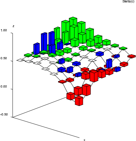
$\begin{figure}\centerline{\hbox{ \psfig{figure=sbars.ps,width=6cm} }} \end{figure}$

Example (ex7.18): This example is similar to the previous one, but now the bars are displayed as vertical towers.

...
NDA> mkgrp win1 -s s1
NDA> setgdat win1 -d sta
NDA> setgcld win1 -c c1
NDA> layer win1 -l 4
NDA> axis win1 -ax z -sca abs -min -0.5 -max 1 -step 4
NDA> nplc win1 -ax z -f s1_W.b_w
NDA> nsize win1 -v 0.5
NDA> topo win1 -on
NDA> bar win1 -f s1_W.crim_w -co red -expr 's1_W.crim_w' > 0.01;
NDA> bar win1 -f s1_W.zn_w -co green -expr 's1_W.zn_w' > 0.01;
NDA> bar win1 -f s1_W.chas_w -co blue -expr 's1_W.chas_w' > 0.01;
NDA> dis win1 barlab barflat saxis
NDA> en win1 bar barvert
NDA> viewp win1 -dz 150 -dy -15 -xy 42 -yz -70
...

$\begin{figure}\centerline{\hbox{ \psfig{figure=vertbars.ps,width=10cm} }} \end{figure}$

Range plots in subgraphs

rngplt Create a range plot

<graphic> name of the graphic structure

-n <name> name for the range plot

-f <field> [-f <field> ...] source fields

[-inx <index>] place of the plot related to others, default=0

[-sca <scaling>] scaling function, default=SOM

[-min <min>] minimum value

[-max <max>] maximum value

-co <color> color for the range lines

[-labs] show values as labels with the plot

rngplt <graphic> -n <name> -rm

Remove a range plot

This command creates range plots to all subgraphs in a graphic structure. The places of the plots related to each other are defined by <index>. The source of the plot includes one or more fields, which are given with the flag -f. The scaling follows the general guides specified in section 8.5. Note that the fields values are sorted automatically. So you need not take care of the order of the fields given for the command.

Example (ex7.19): The following commands create plots for displaying the average values (crim_min, crim_max) and (zn_min, zn_max) in a SOM-oriented graphic structure.

...
NDA> clstat -c cld -d boston -dout stadata -all
...
NDA> mkgrp grp1 -s som
...
NDA> rngplt grp1 -n crim -f stadata.crim_min -f stadata.crim_max
      -sca data -min boston.crim -max boston.crim -co red
NDA> rngplt grp1 -n zn -f stadata.zn_min -f stadata.zn_max
      -sca data -min boston.zn -max boston.zn -co blue

$\begin{figure}\centerline{\hbox{ \psfig{figure=rngplt.ps,width=10cm} }} \end{figure}$

Line diagrams in subgraphs

ldgr Create an empty line diagram

<graphic> name of the graphic structure

-n <name> name of the line diagram

-co <color> color for the line diagram

ldgr <graphic> -n <name> -rm

Remove a line diagram

ldgrc Set the component of a line diagram to all subgraphs

<graphic> name of the graphic structure

-n <name> name of the line diagram

-inx <index> index of the component

-f <field> source field

[-sca <scaling>] scaling function, default=SOM

[-min <min>] minimum value

[-max <max>] maximum value

ldgrcld Set the component of a line diagram to all subgraphs

<graphic> name of the graphic structure

-n <name> name of the line diagram

-inx <index> index of the component

[-id <subgraph>] the idendifier of a subgraph

-f <field> source field

-c <cldata> a classified data

[-sca <scaling>] scaling function, default=SOM

[-min <min>] minimum value

[-max <max>] maximum value

[-rand <percents>] percepts of the randomness around the points (0-100)

The first command ldgr creates empty line diagrams to all subgraphs. Then, commands ldgrc or ldgrcld can be used to add components to these diagrams. ldgrc sets the components of the line diagram according to one data record that has been associated to a subgraph. Instead, ldgrc gets fields through a classifying data frame <cldata> from which a class associated to a subgraph is used to determine the data records from data. Thus, the number of classes in a classifying data frame should be equal to the number of subgraphs. If the random factor (-rand) is given, the lines are scattered according to the percentual value. To remove the line diagram components, the whole line diagram should be deleted.

Example (ex7.20): This example displays three line diagrams in two subgraphs. First the line diagrams are created and then three components are added into them.

...
NDA> mkgrp grp1
NDA> addsg grp1
NDA> setsg grp1 -inx 0 -rec 15
NDA> addsg grp1
NDA> setsg grp1 -inx 1 -rec 50
NDA> ldgr grp1 -n l1 -co red
NDA> ldgrc grp1 -n l1 -inx 0 -f boston.zn
NDA> ldgrc grp1 -n l1 -inx 1 -f boston.age
NDA> ldgrc grp1 -n l1 -inx 2 -f boston.rate

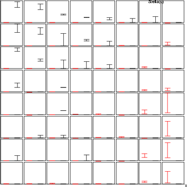
$\begin{figure}\centerline{\hbox{ \psfig{figure=ldgr.ps,width=6cm} }} \end{figure}$

Example (ex7.21): This second example shows, how line diagrams can be used to display the ranges of data in neurons. Two line diagrams min and max are created and then three components zn_min, age_min, rate_min are set to the diagram min and the corresponding maximum values are set to the diagram max.

...
NDA> clstat -c cld1 -d boston -dout stadata -all
...
NDA> mkgrp grp1 -s som
...
NDA> ldgr grp1 -n min -co red
NDA> ldgrc grp1 -n min -inx 0 -f stadata.zn_min -sca data
      -min boston.zn -max boston.zn
NDA> ldgrc grp1 -n min -inx 1 -f stadata.age_min -sca data
      -min boston.age -max boston.age
NDA> ldgrc grp1 -n min -inx 2 -f stadata.rate_min -sca data
      -min boston.rate -max boston.rate
NDA> ldgr grp1 -n max -co blue
NDA> ldgrc grp1 -n max -inx 0 -f stadata.zn_max -sca data
      -min boston.zn -max boston.zn
NDA> ldgrc grp1 -n max -inx 1 -f stadata.age_max -sca data
      -min boston.age -max boston.age
NDA> ldgrc grp1 -n max -inx 2 -f stadata.rate_max -sca data
      -min boston.rate -max boston.rate
...

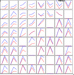
$\begin{figure}\centerline{\hbox{ \psfig{figure=sldgr.ps,width=8cm} }} \end{figure}$

Example (ex7.34): This third example shows, how all data records classified to the neurons can be plotted. The presentation is also known as parallel coordinates.

...
NDA> mkgrp grp1 -s som
...
NDA> ldgr grp1 -n set1 -co red
NDA> ldgrcld grp1 -n set1 -inx 0 -f boston.zn -c cld -sca data
      -min boston.zn -maxboston.zn
NDA> ldgrcld grp1 -n set1 -inx 1 -f boston.age -c cld -sca data
      -min boston.age -max boston.age
NDA> ldgrcld grp1 -n set1 -inx 2 -f boston.rate -c cld -sca data
      -min boston.rate -max boston.rate

$\begin{figure}\centerline{\hbox{ \psfig{figure=ldgrcld.ps,width=8cm} }} \end{figure}$

Line diagrams based on the values of the field

ldgrv Create a line diagram for a vector in one subgraph

<graphic> name of the graphic structure

[-inx <index>] index of the subgraph

-f <field> source field

-co <color> color for the line diagram

[-sca <scaling>] scaling function

[-min <min>] minimum value

[-max <max>] maximum value

ldgrv <graphic> -f <field> -rm

Remove a line diagram from a field

This operation creates a subgraph and computes a line diagram from the values of a field. The indexes of data records are placed into the x axis, and their values are presented in the y axis. If the subgraph identified by <index> does not exist, first the operation creates a new one.

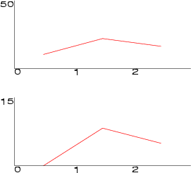
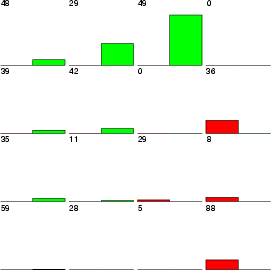
Example (ex7.22): Two fields crim and zn are described with line diagrams in the lower subgraph. Data field age is displayed in the upper subgraph.

NDA> load boston.dat
NDA> mkgrp grp1
NDA> ldgrv grp1 -inx 0 -f boston.crim -co red
NDA> ldgrv grp1 -inx 0 -f boston.zn -co green
NDA> ldgrv grp1 -inx 1 -f boston.age -co blue
NDA> show grp1

$\begin{figure}\centerline{\hbox{ \psfig{figure=ldgrv.ps,width=9cm} }} \end{figure}$

Histograms in subgraphs

hst Create a histogram

<graphic> name of the graphic structure

[-inx <index>] place of the bar related to others

-d <field> source field or data frame

[-x <xaxis>] field for defining the x axis

[-sca <scaling>] scaling function, default=DATA

[-min <min>] minimum value

[-max <max>] maximum value

[-co <color>] color for the histogram bars

hst <graphic> -d <data> -rm Remove a histogram

This command sets a histogram for subgraphs. The actual histogram data can be computed with fldhisto and clhisto (see sections 4.7.3 and 4.8.6). These commands produce two different formats for histogram data, which must be taken into account when a graphical presentation is created.

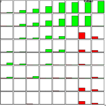
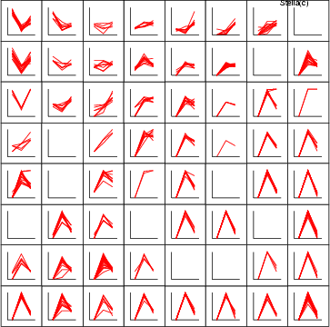
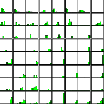
fldhisto: This command creates a frame with two fields: x and N. Thus the command hst should refer to field N. After one histogram has been created, the index must be specified.
clhisto: This command creates a data frame, in which a class (neuron) has one data record and each bin of the histogram is stored in its own field. These fields are named with running numbers from 0 to bins1. In addition, the histogram is a frame containing this data frame called data and a field for the x axis named x. hst does not require parameter -index. All the subgraphs will get a histogram. Of course, this command requires that a graphic structure has a subgraph for each class as SOM based graphics should always have.

Example (ex7.23): This example shows, how histograms can be set for each neuron in a SOM.

# SOM training and classification
...
NDA> clhisto -c c1 -max 10 -f boston.age -dout hst
NDA> mkgrp grp1 -s s1
NDA> layer grp1 -l 3
NDA> hst grp1 -d hst.data -co red -sca som2

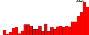
$\begin{figure}\centerline{\hbox{ \psfig{figure=hst.ps,width=8cm} }} \end{figure}$

Example (ex7.24): This second example shows, how a simple histogram can be computed for one field. For another example, see the description of command fldhisto in section 4.7.3.

# SOM training and classification
...
NDA> fldhisto -f boston.age -max 30 -dout fhst
NDA> mkgrp grp
NDA> addsg grp
NDA> hst grp -inx 0 -d fhst.N -co red

$\begin{figure}\centerline{\hbox{ \psfig{figure=fhisto.ps,width=8cm} }} \end{figure}$

The curves of the functions

func1 Set a curve for fuzzy basis functions

<graphic> name of the graphic structure

[-inx <index>] index of the subgraph, default for all

-f <field> source field including function description

[-co <color>] color for the histogram bars

func1 <graphic> [-inx <index>] -f <field> -rm

Remove function curves

This command sets curves for fuzzy basis functions. The shapes of the functions are specified in a field. The command can display only three function types: triangular, trapetzoidal and smoothed trapetzoidal. More information about them and examples can be found in section 4.9.3.

Field labels and values as text in subgraphs

rlab Set labels for subgraphs

<graphic> name of the graphic structure

-n <rulename> name of the rule

-expr <b.expr> boolean expression

rlab <graphic> -n <name> -rm

Remove rule labels

fval Set field values for subgraphs

<graphic> name of the graphic structure

-f <field> source field

-len <len> the length of the label of the value

fval <graphic> -f <field> -rm Remove field values for field

These two commands are used for displaying the values of the fields as text. The command rlab shows the name of the rule in those subgraphs, which fulfill the rule. The command fval shows values as text in neurons. These commands only work with SOM oriented graphic structures at the moment.

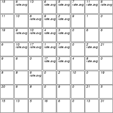
Example (ex7.25): In this example, the variable hits is displayed as text. Then those neurons, in which the value of rate_avg is within range [25, 50], are labelled.

...
NDA> clstat -c cld -d boston -dout stadata -all
NDA> mkgrp grp1 -s som
...
NDA> layer grp1 -l 3
NDA> fval grp1 -f stadata.hits
NDA> rlab grp1 -n stadata.rate_avg -expr 25 <= 'stadata.rate_avg'
      AND 'stadata.rate_avg' <= 50;

$\begin{figure}\centerline{\hbox{ \psfig{figure=flab.ps,width=8cm} }} \end{figure}$

Record labels in subgraphs

reclab Set record labels for subgraphs

<graphic> name of the graphic structure

-f <field> source field

[-l <layer>] layer to be labelled

[-max <max>] maximum number of the labels in each subgraph

[-c <cldata>] an optimal classified data

reclab <graphic> -rm Remove record labels

This command displays the values of some field in subgraphs. The labels are read from the specified field. The layer to be labelled and the maximum number of labels in each neuron can be restricted with <layer> and <max>. <cldata> should contain associations between data records and subgraphs. If <cldata> is not specified, then the classified data, that has been connected to the graphic structure with setgcld, is used.

Example (ex7.26): The values of field crim are picked from Boston data and placed into neurons.

...
NDA> mkgrp grp1 -s som
NDA> setgcld grp1 -c cld
NDA> layer grp1 -l 3
NDA> reclab grp1 -f boston.crim -l 3

$\begin{figure}\centerline{\hbox{ \psfig{figure=reclab.ps,width=12cm} }} \end{figure}$

Data matrix in subgraphs

pmat set a data matrix for subgraphs

<graphic> name of the graphic structure

-n <name> name of the point matrix

-id <subgraph> the idendifier of a subgraph

-d <data> data to be displayed

[-sca <scaling>] scaling function, default=DATA

[-min <min>] minimum value

[-max <max>] maximum value

[-co <color>] color for the histogram bars

[-rgb] colors are displayed as pseudo colors

pmat <graphic> -n <name> -id <subgraph> -rm Remove a data matrix

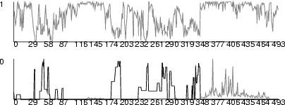
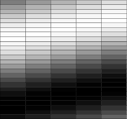
This command displays the values of the given data in a subgraph as a matrix. One row corresponds to one data record, and one column to one field, respectively. The values are displayed as gray levels or pseudo colors, depending on the flag -rgb. The scaling parameters define how the values are mapped to the colors. The values can be either integer or floating points.

Example (ex7.35): The following commands generate data using a sine function, create sequences of the values and show the sequences in the data matrix.

NDA> setdata -f d.i -vals 0=0.0; -t float -len 30
NDA> serie -d d -fout d.x
NDA> expr -fout d.x -expr 2 * 3.14 * FLOAT('d.x') / LEN("d.x");
NDA> expr -fout d.y -expr SIN('d.x');
NDA> select data -f d.y
NDA> concseq -d data -dout data1 -len 5
NDA> mkgrp win1
NDA> addsg win1
NDA> pmat win1 -n rm -id 0 -d data1
NDA> en win1 pmat

$\begin{figure}\centerline{\hbox{ \psfig{figure=pmat.ps,width=4cm} }} \end{figure}$

Vector fields

vecfld set a vector field to the graphics

<graphic> name of the graphic structure

-n <name> name of the point matrix

-d <data> data to be displayed

[-fw <field>] the field holds width of the vectors

[-fb <field>] field of the start points

[-fe <field>] field of the end points

[-co <color>] color of the vectors

vecfld <graphic> -n <name> -rm

Remove a vector field

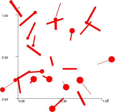
The command sets a vector field to the graphics. The vectors can be defined through their coordinates, width, sizes of the starting and ending points and their color. The coordinates are given in a mandatory parameter <data>. It must have six fields: three first fields are coordinates of the starting points, and three last fields holds coordinates of the ending points. The scales of the values is the unit cubic . Note that vector fields does not depend on axis settings.

The optional parameters with the flags -fb and -fe describe sizes of the start and end points. Their scales are also in the range [0,1], indicating that the point with the value 1 fills the unit cubic. Therefore, typical values for these parameters are about 0.01.

The vector width is given in the field with the flag -fw. The width is a relative value where the value 0 means the minimum width, and the scale depends on the implementation of the graphic display. Note that the graphic display does not necessarily support this feature.

Example (ex7.36): The following commands generate random data and displays it as a vector field. The figure below shows two displays: in the first (PostScript) the width of the links is constant, while in the second one the display can change the width (Xview).

# Create a random data
#
NDA> setdata -f i -vals 0=0; -t float -len 25
NDA> expr -fout vdat.x1 -expr 'i' - 'i' + RAND(1.0);
NDA> expr -fout vdat.y1 -expr 'i' - 'i' + RAND(1.0);
NDA> expr -fout vdat.z1 -expr 'i' - 'i';
NDA> expr -fout vdat.x2 -expr 'vdat.x1' + RAND(0.4) + -0.2;
NDA> expr -fout vdat.y2 -expr 'vdat.y1' + RAND(0.4) + -0.2;
NDA> expr -fout vdat.z2 -expr 'i' - 'i';
NDA> serie -d vdat -fout x -start 1 -step 0
NDA> expr -fout p -expr 'i' - 'i' + RAND(1.0) / 25.0;
NDA> expr -fout q -expr 'i' - 'i' + RAND(10.0);
#
# Create graphics and set the axis scales
#
NDA> mkgrp win1
#
NDA> axis win1 -ax x -sca abs -min 0.0 -max 1.0 -step 3
NDA> axis win1 -ax y -sca abs -min 0.0 -max 1.0 -step 3
#
# Set the vector field
#
NDA> vecfld win1 -n v -d vdat -co red -fe p -fw q
#
# Enable the vector field in the low level graphics
#
NDA> en win1 vecfld axis
NDA> viewp win1 -dz 150

$\begin{figure}\centerline{\hbox{ \psfig{figure=vecfld.ps,width=9cm} }} \end{figure}$

Colors and scaling

Colors

Basic colors may be specified as names or numbers. Allowed names are listed below and, if a number is specified, it is reduced into range [0,MAX_COL-1] by taking the remainder of integer division by MAX_COL. random provides a randomly selected basic color.

Names of the colors:

red, green, blue, yellow, magenta, orange, cyan, brown, black, white

random

In addition, some operations might use gray levels or colors of the warm color scale, which are coded as data field values between 0 and 255. The choice between the gray and color scales can be chosen in those commands with -rgb switch. To use the gray levels or warm scale colors for neurons, bars, data points, groups, etc. the following notations can be used:

gray_<n> Selects the <n>th color of the gray

scale $0 \leq n \leq 255$ (black ... white)

rgb_<n> Selects the <n>th color of the warm

scale $0 \leq n \leq 255$ (blue ... red)

gray_random Selects a random color of the gray scale

rgb_random Selects a random color of the warm color scale

Example: For instance, color can be specified to the following commands.

...
NDA> bar grp1 -f crim -co red
NDA> bar grp1 -f zn -co rgb_220
NDA> gcolor grp1 -cl g1 -co red

Scaling

The scaling functions:

data find the range of a data vector

abs absolute values given as parameters

vec select corresponding minimum and maximum components from the vectors given as parameters

som find minimum and maximum values inside the SOM (TS-SOM layer)

som2 like som, but empty neurons are skipped

The scaling plays a key role when values from data frames are converted into features of graphical objects. Five functions for scaling values are listed above. The first three functions can be used with any type of graphic structure, som and som2 only work with the SOM-oriented graphic structure.

Example (ex7.27): The following commands demonstrate briefly the use of scaling.

...
NDA> mkgrp grp1 -s s1
NDA> setgdat grp1 -d stadata
# Default scaling is typically "data"
NDA> bar grp1 -f stadata.crim_avg -co red
# Use the range of the field inside the current layer of TS-SOM
NDA> bar grp1 -f stadata.crim_avg -co red -sca som
# Similar to the previous command, but skip empty neurons
NDA> bar grp1 -f stadata.crim_avg -co red -sca som2
...

Graphics for groups in a SOM

This command is meant for displaying the grouping of neurons.

gcolor Set a color for a group

<graphic> name of the graphic structure

-cl <class> name of a group (class in a classified data)

-co <color> color to be used

gcolor <graphic> -cl <group> -rm

Clear the color and labels from a group

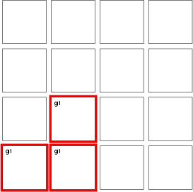
This command sets the colors and inserts labels to the neurons belonging to a specified group <class>.

Example (ex7.28): The example sets a color for the group g1.

...
NDA> mkgrp grp1 -s s1
NDA> setgcld grp1 -c cld1
...
NDA> addcld -c groups
NDA> addcl -c groups -cl g1
NDA> updcl -cl groups.g1 -id 5
NDA> updcl -cl groups.g1 -id 6
NDA> updcl -cl groups.g1 -id 8
...
NDA> layer grp1 -l 2
NDA> gcolor grp1 -cl groups.g1 -co red

$\begin{figure}\centerline{\hbox{ \psfig{figure=glab.ps,width=6cm} }} \end{figure}$

Adding custom graphic elements

These commands add custom graphic elements, which are not tied to a subgraph. Instead, the position for these shapes is specified using global (x, y, z) coordinates. Several texts, polygons and ellipses can be defined by using unique element names.

Defining custom graphic texts

freetext Defines a custom graphic text

<graphic> name of graphic

-n <name> name for text element

-fco <fco> foreground color

-x <x> x location

-y <y> y location

-z <z> z location

-t <text> text

freetext <graphic> [-n <name>] -rm

remove specified text element(s)

Name of the graphic is specified using <graphic>, whereas name for the custom text element is given in <name>. Foreground color must be specified using <fco> and the location of text is set by the (<x>, <y>, <z>) triple. Text to be displayed is given in <text> (use double quotes, if needed). -rm can be used for removing either the named text element or all text elements (if <name> is omitted) from the graphic.

Example:

NDA> mkgrp win1
NDA> freetext win1 -n text1 -fco black -x 0.80 -y 0.9 \
     -z -100.0 -t text
NDA> freetext win1 -n text2 -fco yellow -x 0.60 -y 0.4 \
     -z -100.0 -t hello
NDA> freetext win1 -n text3 -fco blue -x 0.60 -y 0.3 \
     -z -100.0 -t world
NDA> show win1

Defining custom graphic polygons

freepolygon Defines a custom graphic polygon

<graphic> name of graphic

-n <name> name for polygon

-d <data> data frame

-fco <fco> foreground color

-bco <bco> background color

freepolygon <graphic> [-n <name>] -rm

remove specified polygon(s)

Name of graphic is specified by <graphic>, whereas name for custom polygon is set by <name>. A data frame containing the 3D coordinates for the corners must be given in <data>. The data frame must contain three floating point fields, which are interpreted as x, y and z coordinates. The names of the fields need not be specific, but the types have to be float. The number of data points specifies the number of corners. The foreground and background colors of the polygons must be specified with <fco> and <bco>. -rm can be used for removing either a named polygon or all polygons (if <name> is omitted) from the graphic.

Example:

NDA> mkgrp win1
NDA> gen -U 0.1 0.3 -dout data3 -dim 3 -s 3
NDA> freepolygon win1 -n poly3 -d data3 \
     -fco black -bco yellow
NDA> gen -U 0.2 0.4 -dout data4 -dim 3 -s 4
NDA> freepolygon win1 -n poly4 -d data4 \
     -fco black -bco blue
NDA> gen -U 0.5 0.9 -dout data10 -dim 3 -s 10
NDA> freepolygon win1 -n poly10 -d data10 \
     -fco black -bco cyan
NDA> show win1

Defining custom graphic ellipses

ellipse Defines a custom graphic ellipse

<graphic> name of graphic

-n <name> name for ellipse

-fco <fco> foreground color

-bco <bco> background color

-x <x> x location

-y <y> y location

-z <z> z location

-rx <rx> radius in x direction

-ry <ry> radius in y direction

-rz <rz> radius in z direction

ellipse <graphic> [-n <name>] -rm

remove specified ellipse(s)

Name of graphic is specified with <graphic>, whereas the name for the ellipse is given using <name>. Foreground and background colors must be given using <fco> and <bco>. The location of the center of the ellipse is specified with the (<x>, <y>, <z>) triple and the size (radii) with <rx>, <ry> and <rz>. ellipse does not draw perspective corrected diagonal ellipses into regular NDA graphs. True 3-D ellipses are only drawn into the OpenGL window. -rm can be used to remove either the named ellipse or all ellipses (if name is omitted) from the graphic.

Example:

NDA> mkgrp win1
NDA> ellipse win1 -n oval1 -x 0.5 -y 0.5 -z 0.0 \
     -rx 0.1 -ry 0.1 -rz 0.1 -fco red
NDA> ellipse win1 -n oval2 -x 0.5 -y 0.5 -z 0.5 \
     -rx 0.2 -ry 0.2 -rz 0.2 -fco blue
NDA> ellipse win1 -n oval3 -x 0.25 -y 0.25 -z -0.5 \
     -rx 0.1 -ry 0.3 -rz 0.2 -fco green
NDA> show win1

Setting a viewpoint to a graphic image in 3D

viewp Set a viewpoint to a graphic image

<graphic> name of the graphic structure

-xy <xy-angle> angle in the xy plane (degrees)

-yz <yz-angle> angle in the yz plane (degrees)

-dx <dx> offset in the x direction

-dy <dy> offset in the y direction

-dz <dz> distance in the z direction, default=100

This operation sets a viewpoint to a graphic image. It uses two angles and three offsets in the direction of each axis. Although the command is used with a SOM-oriented graphic structure in the following example, it can also be used with any 3D graphic structure.

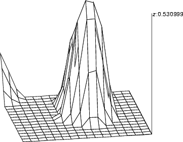
Example (ex7.29): This example shows how a SOM-oriented graphic structure can be viewed from different angles. Axis z is used for displaying the weight chas_w while the axes x and y are spanned according to the grid of the SOM. The shape of the neurons is changed to polygon to achieve a smoother surface.

...
NDA> somtr -d predata -sout som -l 5
...
NDA> mkgrp grp1 -s som
NDA> layer grp1 -l 4
NDA> nshape grp1 polygon
...
NDA> viewp grp1 -dz 150 -xy -100 -yz -70

$\begin{figure}\centerline{\hbox{ \psfig{figure=viewp.ps,width=8cm} }} \end{figure}$

Displaying an image in a window

bgimg Display an image in a window

<graphic> name of the graphic structure

-img <name> image name in namespace

[-x0 <x-coord>] x-coordinate of a portion

[-y0 <y-coord>] y-coordinate of a portion

[-w <width>] width of a portion

[-h <height>] height of a portion

bgimg <graphic> -rm Remove existing image from a window

This command can be used to add an image to be drawn on the background of a window. Switches -x0, -y0, -w and -h can be used to specify a portion to be used instead of the whole picture.

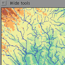
Example: In this example an image file is loaded and a portion of it is visualized in a window.

...
# Load the image file into namespace
NDA> loadimg map.gif
# Create a graphic structure and assign a 300 by 300 pixel portion
# of the image starting at (100, 100)
NDA> mkgrp win
NDA> bgimp win -img map -x0 100 -y0 100 -w 300 -h 300
NDA> show win
...
# Remove the background image
NDA> bgimg win -rm
NDA> draw /win

$\begin{figure}\centerline{\hbox{ \psfig{figure=bg_map.ps,width=5cm} }} \end{figure}$

Displaying graphics

These commands are meant for selecting components for a presentation. This does not lead to recomputing, but it has an effect only on a low level image.

en Enable components to be displayed

dis Disable components to be displayed

<graphic> name of the graphic structure

<mode-1> [... <mode-n>] selected components

<mode-i> $\in$ {fg, bg, axis, saxis, datplc, ndatplc, cntr, cntrlab, bar, hst, ldgr, rlab, fval, reclab, glab, gcolor, gfill}

These commands select the components of a graphic structure, which are to be displayed or dropped out from the final presentation. These commands work as a quick selection of features and do not affect the settings of the graphic structure, which are defined, for instance, with commands bar or rlab (see sections 8.4.3 and 8.4.9), even if bars are disabled.

Parameters <mode-i> define, which components are displayed. The mode works in a hierarchical manner. The main level defines the component types, which are to be shown. In addition, there are additional subtypes for, for instance, bars, with which the detail level of the final presentation can be selected.

Main level for <mode-i>

fg frame for subgraphs

bg background for subgraphs

axis main axes for a 3D display

saxis axes for each subgraph

datplc data scattering in 3D

ndatplc data scattering inside neurons

cntr contours

cntrlab labels for contours

bar bars

rngplt range plot

hst histograms

ldgr line diagrams

rlab labels for rules

fval field values in subgraphs

pmat point matrix in sungraphs

vecfld vector fields

reclab record labels

glab group labels

gcolor group colors

gfill group filling

<mode-i> types for bars

barflat 2D bars

barvert 3D bars as towers

barlab labels for bars in each subgraph

barlab1 labels for bars only in the first subgraph

<mode-i> types for line diagrams

ldgrlab labels for line diagrams

<mode-i> types for range plots

rngval show values with the plot

rnglab show names of the plots

Example (ex7.30): This short example shows, how the commands can be used.

...
NDA> mkgrp grp1 -s s1
...
# Show all components
NDA> en grp1 all
...
# Hide the frame of the neurons, but display their contents
NDA> dis grp1 fg barvert barlab barlab1
...

$\begin{figure}\centerline{\hbox{ \psfig{figure=dis.ps,width=6cm} }} \end{figure}$

Querying the settings of a graphic structure

getg Return the settings of a graphic structure

<graphic> name of the graphic structure

[<command>] command for the graphic structure

<command> $\in$ {layer, topo, cntr, traj, axis, saxis, ndiam, nshape, nsize, nplc, nvsbl, ncolor, ngray, nconn, umat, sons, bar, rngplt, rlab, fval, gcolor, datplc, hst, ldgr, ldgrc, ldgrcld, ldgrv, vecfld, pmat, en, viewp}

<command> $\in$ {src, scales, colors}

[-dout <data>] output data

[-fout <field>] output field

This command is meant for querying the settings of a graphic structure as commands. If parameter <command> has been omitted, then the whole state is returned. One can store results in a data frame and field using the parameters <data> and <field>. Their use is described below with various command settings.

<command> Returned data - Commands for selecting or setting...

layer the layer

topo the topology of the TS-SOM

cntr the contours on the TS-SOM layer

traj the trajectory on the TS-SOM layer

axis the axes

saxis the subaxes

ndiam the diameter of circles of the neurons

nshape the shape of the neurons

nsize the size of the neurons

nplc the location of neurons

nvsbl the neuron visibility

ncolor the color of the neurons

ngray the gray level of the background of the neurons

nconn the neuron connectors

umat the U-matrix presentation

sons the son links

bar the bars

rngplt the range plots

rlab the labels in the subgraphs

fval field values

gcolor the color of the group

datplc the data vector related to the axis

hst histograms

ldgr, ldgrc, ldgrv line diagrams

vecfld the vector field

pmat the point matrix

viewp the viewpoint to the graphic image

en commands for enabling components to be displayed

If the field (and data) is given, then the results are stored in the field. Otherwise, the output is directed to the output stream.

The flags src, scales and colors do not return commands. Instead they return data as follows.

<Other commands>

src Return names of the selected sources of data (stored in the graphic structure): SOM, data frame and classified data

scales Return the scales of graphical objects (minimum and maximum values). This flag requires an option to specify the type of objects to be queried. Possible options are axis, saxis, ndiam, ngray, bar, rngplt, ldgrc, ldgrcld, ldgrv, pmat

colors Return the colors of graphical objects (foreground and background colors). This flag requires an option to specify the type of objects to be queried. Possible options are bar, rngplt, ldgr, ldgrv, hst, gcolor, dtaplc, ndatplc, traj, cntr, vecfld

If the parameter <data> is given, then the scales and colors are stored in this data. The scales are stored in data that have three fields: name, min and max. Respectively, the colors will be stored in data that have three fields: name, fg and bg. The name refers to the parameter that identifies the graphic setting. The command src always results the output stream.

Example (ex7.31): First, run the example `ex7.31'. Then apply command getg.

...
NDA> mkgrp grp1 -s s1
...
NDA> getg grp1 bar
bar grp1 -inx 0 -f sta.crim_avg -co red -sca data 
bar grp1 -inx 1 -f sta.zn_avg -co green -sca abs  -min 10.000000
     -max 100.000000
NDA> getg grp1 axis
axis grp1 -ax x -f som_x -sca abs  -min 0.000000 -max 1.000000
 -step 3 
axis grp1 -ax y -f som_y -sca abs  -min 0.000000 -max 1.000000
 -step 3 
axis grp1 -ax z -f som_z -sca abs  -min 0.000000 -max 1.000000
 -step 3
NDA> getg grp1 scales bar
sta.crim_avg
0.000000
66.142067
sta.zn_avg
10.000000
100.000000
NDA> getg grp1 scales bar -dout bar_scales
NDA> getg grp1 -fout graphics_commands

Saving the settings of a graphic structure into a file

savegrp Save the settings of a graphic structure as commands

<graphic> name of the graphic structure

-o <filename> output file

This command writes the settings of a graphic structure into a file as commands. If there is no specified settings, the returned data will be empty. (See the example in section 8.11).

...
NDA> mkgrp grp1 -s s1
...
NDA> savegrp grp1 -o cmds.txt

Graphic frames

Creating a graphic frame

mkgf Create a graphic frame

-gf <gframe> name for the graphic frame

This command creates an empty graphic frame, to which graphic structures can be connected with addgf.

Adding a graphic structure to a graphic frame

addgf Add a graph to a graphic frame

-gf <gframe> name of the graphic frame

-g <graphic> name of the graph

[-noname] remove the name of the graphic structure from the frame

This command connects a graphic structure into a graphic frame. If -noname is specified, the name of the graphic structure is omitted from the graphic frame. The default is to show the name underneath the graph.

Setting the places of graphic structures within graphic frames

setgfplc Set the place of a graphic structure within a graphic frame

-gf <gframe> name of the graphic frame

-g <graphic> name of the graphic structure

[-x0 <x0>] left boundary in [0,1], default = 0.0

[-y0 <y0>] bottom boundary in [0,1], default = 0.0

[-x1 <x1>] right boundary in [0,1], default = 1.0

[-y1 <y1>] top boundary in [0,1], default = 1.0

[-noname] remove the name of the graphic

[-name] show the name of the graphic structure

This command sets the place of a graphic structure related to a graphic frame. The ranges of the coordinates are in . -noname forces the name of the graphic structure not to be shown in the frame, and -name makes sure that it will be shown (if hidden earlier with addgf or setgfplc).

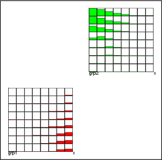
Example (ex7.32): Two graphic structures are created and then connected to a graphic frame. They are further placed within the frame.

NDA> mkgrp grp1 -s som
NDA> mkgrp grp2 -s som         # ... and define bars in them
NDA> mkgf -gf frm1             # Create a frame and set it
NDA> addgf -gf frm1 -g grp1
NDA> setgfplc -gf frm1 -g grp1 -x0 0.05 -y0 0.05 -x1 0.45 -y1 0.45
NDA> addgf -gf frm1 -g grp2
NDA> setgfplc -gf frm1 -g grp2 -x0 0.55 -y0 0.55 -x1 0.95 -y1 0.95
NDA> show frm1 -t frm

$\begin{figure}\centerline{\hbox{ \psfig{figure=gframe.ps,width=7cm} }} \end{figure}$

Commands for working with low level images

These commands are meant for generating low level images and for mapping events to them.

Generating a low level image from a graphic structure

setimg Generate a low level image

<graphic> name of the graphic structure

[-t <type>] type of view: net | vec

rmimg Clear a low level image

<graphic> name of the graphic structure

These commands can be used to generate and clear a low level graphic structure. The low level image is a list of graphical primitives, which can be displayed with simple graphic routines. Normally these commands are embedded within other commands such as wrps (see section 9.3) or the user interface.

...
NDA> mkgrp grp1 -s s1
...
NDA> setimg grp1
...
NDA> rmimg grp1

Finding objects from a graphic structure

fndpnt Find a graphical object for a specified point

<graphic> name of the graphic structure

<x> <y> x and y values, normally between [0,1]

fndreg Find graphical objects inside a specified region

<graphic> name of the graphic structure

<x1> <y1> ... <xn> <yn> (x, y) pairs

These commands are used to return the identifiers of graphical objects, which are close to a specified point or inside a spcified region. The result actually contains the identifiers of the owners of those objects. Neurons' id numbers, for instance.

The objects are located from a low level image and, thus, the coordinates given to the command are typically in the space . In practice, points for this procedure are received from mouse events.

Example: A graphic structure has been created and layer 2 selected to be displayed. Then the topmost object for the point (0.2, 0.2) is located. Secondly, all the objects with different owners are located from the region, which is located in the bottom-left corner of the graphic structure. See also the second example in section 2.13. You should first run the example `ex7.4' and then apply commands fndpnt and fndreg.

...
NDA> mkgrp grp1 -s s1
NDA> layer grp1 -l 2
...
# Locate the topmost neuron from point (0.2, 0.2).
NDA> fndpnt grp1 0.2 0.2
5
...
# Locate neurons from a given region
NDA> fndreg grp1 0.1 0.1 0.5 0.1 0.5 0.5 0.1 0.5
8
6
5
7
...

Executing macros according to a selection within a graphic structure

runevent Find a graphical object for a given point and run a macro

<graphic> name of the graphic structure

-mac <macro>; macro and its parameters

<x1> <y1> ... <xn> <yn> (x, y) pairs

This command executes the specified macro for all the objects inside a region defined with (, ) points. If only one point has been specified, then an object closest that point is located. If several points have been specified, those points are interpreted as corner points of a region and all objects inside that region are located. Located objects are converted into the identifiers of the owners of the objects, and then for each identifier the macro is executed in the following manner:

runcmd <macro> <graphic> <id>

The objects are located from a low level image and, thus, the specified coordinates are typically within the space . In practice, the points for this procedure are received from mouse events.

Note that after the <macro> name you must put a `;'. Thus you can also specify additional parameters for the macro.

Example: A graphic structure has been created and layer 2 selected to be displayed. Then the topmost object for point (0.2, 0.2) is located and macro selectNeuron is executed.

...
NDA> mkgrp grp1 -s s1
NDA> layer grp1 -l 2
...
NDA> runevent grp1 -mac selectNeuron; 0.2 0.2

The macro selectNeuron can select neurons into a classified data (grouping of the neurons) as follows:

...
addcld -c $1grp
addcld -c $1grp -cl $1grp.sel
updcld -cl $1grp.sel $2
...

Generating a low level image for a graphic frame (tech.)

setgfimg Generate a low level image

-gf <gframe> name of the graphic frame

This command generates a low level image from a graphic frame.

Updating a graphic structure

updgr Update a graphic structure

<graphic> name of the graphic structure

<mode> <mode> $\in$ {all, bar, ldgr, rngplt, hst, rlab, fval, reclab, gcolor, func1}

This command updates the settings of a chosen graphic structure according to specified flags.

...
NDA> mkgrp grp1 -s s1
NDA> bar grp1 -f sta.crim_avg -co red
NDA> fval grp1 -f sta.zn_avg
NDA> updgr win1 all

Next: File I/O Up: User's reference Previous: Revised image processing commands Contents

Anssi Lensu 2006-02-23

mkgrp	Create a new graphic structure
<graphic>	name for the graphic structure
[{-s <som> \|	a TS-SOM structure
-d <data>}]	a data frame
setgdat	Connect a data frame to graphics
<graphic>	name of the graphic structure
-d <data>	a data frame
setgcld	Connect a classified data frame to graphics
<graphic>	name of the graphic structure
-c <cldata>	a classified data frame

addsg	Create a new subgraph to a graphic structure
<graphic>	name of the graphic structure
setsg	Connect a data record to a subgraph
<graphic>	name of the graphic structure
-inx <index>	index of the subgraph
-rec <recinx>	index of the data record
rmsg	Remove the specified subgraph
<graphic>	name of the graphic structure
-inx <index>	index of the subgraph

layer	Set the layer of TS-SOM
<graphic>	name of the graphic structure
-l <layer>	index of the layer
[-min <min>]	starting layer

topo	Show/hide the topology of TS-SOM
<graphic>	name of the graphic structure
-on \| -off	topology on/off
[-c <cldata>]	classified data for links
[-all]	show all the links
sons	Show/hide child links of the TS-SOM
<graphic>	name of the graphic structure
-on \| -off	child links on/off

traj	Create or set a trajectory
<graphic>	name of the graphic structure
-n <name>	name for the trajectory
-min <min>	starting index of data
-max <max>	ending index of data
-co <color>	color for the trajectory
[-step <step>]	step between the labels
[-f <field>]	field for labelling. If omitted, indexes are used as labels
[-c <cldata>]	another classified data
[-d <ddata>]	distance data, which describes the distances between data records and their BMU neurons
traj <graphic> -n <name> -rm	Remove trajectory <name>

nconn	Connect neurons through external information
<graphic>	name of the graphic structure
-n <name>	name for the connector
-c <cldata>	link information
-min <min>	lower boundary for links
-max <max>	upper boundary for links
[-co <color>]	color for the connector
[-nolab]	if the lines should not be labelled with proportions
nconn <graphic> -n <name> -rm	Remove connector <name>

cntr	Set a contour
<graphic>	name of the graphic structure
-n <name>	name of the contour
-f <field>	field to be used for neurons
-v <value>	value for the contour (elevation)
[-co <color>]	color for the contour
[-t <type>]	how the contour is drawn
cntr <graphic> -n <name> -rm	Remove contour <name>

umat	Set a U-matrix to be used while visualizing a graphic structure
<graphic>	name of the graphic structure
-umat <umat>	name of the U-matrix data to be used
umat <graphic> -rm	Clear the U-matrix presentation

axis	Set an axis
<graphic>	name of the graphic structure
-ax <axis>	name of the axis: x, y or z
[-sca <scaling>]	scaling function
[-f <field>]	field for computing the scale
[-min <min>]	minimum value
[-max <max>]	maximum value
[-step <scales>]	the number of scale labels
axis <graphic> -ax <axis> -rm	Remove axis <axis>

datplc	Scatter the values of a data vector to one axis
<graphic>	name of the graphic structure
-n <setname>	name of the scatterplot
-ax <axis>	name of the axis: x, y or z
-f <field>	data field to be scattered
[-co <color>]	color for data points
[-volume <vol_size>]	size
[-shape <shape>]	shape
[-shape_data <char>]	shape data (for character shape)
datplc <graphic> -n <name> -rm	Remove scatterplot <name>

nplc	Set the places of neurons related to an axis
<graphic>	name of the graphic structure
-ax <axis>	name of the axis: x, y or z
-f <field>	data field for the locations
nplc <graphic> -ax <axis> -rm	Set the neuron locations for one specified axis to 0.0

nshape	Set the shape of the neurons
<graphic>	name of the graphic structure
<shape>	Chosen shape: rectangle \| polygon \| circle
[-expr <expr>;]	a boolean expression

nsize	Set the size of neurons
<graphic>	name of the graphic structure
-v <value>	size for the neurons (usually relative to the SOM grid)
[-abs]	<value> is to be used as an absolute value; otherwise it is relative to the SOM grid (default)

ndiam	Set the diameter of circular neurons
<graphic>	name of the graphic structure
-f <field>	name of the field
[-sca <scaling>]	scaling function
[-min <min>]	minimum value
[-max <max>]	maximum value
ndiam <graphic> -rm	Set relative diameters to 1.0

ncolor	Set the color of neurons
<graphic>	name of the graphic structure
-fg <fgcolor>	foreground color
-bg <bgcolor>	background color
[-expr <expr>;]	a boolean expression
ngray	Set the gray level for the background of the neurons
<graphic>	name of the graphic structure
-f <field>	source field for evaluating gray levels
[-sca <scaling>]	scaling function, default=SOM
[-min <min>]	minimum value
[-max <max>]	maximum value
[-rgb]	use the pseudo colors instead of gray levels

nvsbl	Set the visibility of neurons
<graphic>	name of the graphic structure
-expr <expr>;	boolean expression to be evaluated using the variables in the neurons
[-v]	verbose evaluation

saxis	Show an axis in the subgraphs
<graphic>	name of the graphic structure
-ax <axis>	name of the axis: `x`, `y` or `z`
[-inx <index>]	index of the subgraph
[-sca <scaling>]	scaling function, default=DATA
[-f <field>]	source field
[-min <min>]	minimum value
[-max <max>]	maximum value
[-step <lab-step>]	number of labels
saxis <graphic> -ax <axis> [-inx <index>] -rm
	Remove the axis definition

ndatplc	Set a data field for an axis to enable data plotting
<graphic>	name of the graphic structure
-n <name>	name of the data to be plotted
-ax <axis>	name of the axis: `x`, `y` or `z`
-f <field>	source field
-c <cldata>	a classified data
[-co <color>]	the color of the data points
ndatplc <graphic> -n <name> -rm
	Remove a data set

bar	Create or alter a bar
<graphic>	name of the graphic structure
[-inx <index>]	bar index
-f <field>	source data field
[-sca <scaling>]	scaling function, default=SOM
[-min <min>]	minimum value
[-max <max>]	maximum value
[-co <color>]	color for the bar
[-expr <bool-expr>]	boolean expression
bar <graphic> -f <field> -rm	Remove a bar

rngplt	Create a range plot
<graphic>	name of the graphic structure
-n <name>	name for the range plot
-f <field> [-f <field> ...]	source fields
[-inx <index>]	place of the plot related to others, default=0
[-sca <scaling>]	scaling function, default=SOM
[-min <min>]	minimum value
[-max <max>]	maximum value
-co <color>	color for the range lines
[-labs]	show values as labels with the plot
rngplt <graphic> -n <name> -rm
	Remove a range plot

ldgr	Create an empty line diagram
<graphic>	name of the graphic structure
-n <name>	name of the line diagram
-co <color>	color for the line diagram
ldgr <graphic> -n <name> -rm
	Remove a line diagram
ldgrc	Set the component of a line diagram to all subgraphs
<graphic>	name of the graphic structure
-n <name>	name of the line diagram
-inx <index>	index of the component
-f <field>	source field
[-sca <scaling>]	scaling function, default=SOM
[-min <min>]	minimum value
[-max <max>]	maximum value
ldgrcld	Set the component of a line diagram to all subgraphs
<graphic>	name of the graphic structure
-n <name>	name of the line diagram
-inx <index>	index of the component
[-id <subgraph>]	the idendifier of a subgraph
-f <field>	source field
-c <cldata>	a classified data
[-sca <scaling>]	scaling function, default=SOM
[-min <min>]	minimum value
[-max <max>]	maximum value
[-rand <percents>]	percepts of the randomness around the points (0-100)

ldgrv	Create a line diagram for a vector in one subgraph
<graphic>	name of the graphic structure
[-inx <index>]	index of the subgraph
-f <field>	source field
-co <color>	color for the line diagram
[-sca <scaling>]	scaling function
[-min <min>]	minimum value
[-max <max>]	maximum value
ldgrv <graphic> -f <field> -rm
	Remove a line diagram from a field

hst	Create a histogram
<graphic>	name of the graphic structure
[-inx <index>]	place of the bar related to others
-d <field>	source field or data frame
[-x <xaxis>]	field for defining the x axis
[-sca <scaling>]	scaling function, default=DATA
[-min <min>]	minimum value
[-max <max>]	maximum value
[-co <color>]	color for the histogram bars
hst <graphic> -d <data> -rm	Remove a histogram

func1	Set a curve for fuzzy basis functions
<graphic>	name of the graphic structure
[-inx <index>]	index of the subgraph, default for all
-f <field>	source field including function description
[-co <color>]	color for the histogram bars
func1 <graphic> [-inx <index>] -f <field> -rm
	Remove function curves

rlab	Set labels for subgraphs
<graphic>	name of the graphic structure
-n <rulename>	name of the rule
-expr <b.expr>	boolean expression
rlab <graphic> -n <name> -rm
	Remove rule labels
fval	Set field values for subgraphs
<graphic>	name of the graphic structure
-f <field>	source field
-len <len>	the length of the label of the value
fval <graphic> -f <field> -rm	Remove field values for field

reclab	Set record labels for subgraphs
<graphic>	name of the graphic structure
-f <field>	source field
[-l <layer>]	layer to be labelled
[-max <max>]	maximum number of the labels in each subgraph
[-c <cldata>]	an optimal classified data
reclab <graphic> -rm	Remove record labels

pmat	set a data matrix for subgraphs
<graphic>	name of the graphic structure
-n <name>	name of the point matrix
-id <subgraph>	the idendifier of a subgraph
-d <data>	data to be displayed
[-sca <scaling>]	scaling function, default=DATA
[-min <min>]	minimum value
[-max <max>]	maximum value
[-co <color>]	color for the histogram bars
[-rgb]	colors are displayed as pseudo colors
pmat <graphic> -n <name> -id <subgraph> -rm	Remove a data matrix

vecfld	set a vector field to the graphics
<graphic>	name of the graphic structure
-n <name>	name of the point matrix
-d <data>	data to be displayed
[-fw <field>]	the field holds width of the vectors
[-fb <field>]	field of the start points
[-fe <field>]	field of the end points
[-co <color>]	color of the vectors
vecfld <graphic> -n <name> -rm
	Remove a vector field

Names of the colors:
red, green, blue, yellow, magenta, orange, cyan, brown, black, white
random

gray_<n>	Selects the <n>th color of the gray
	scale $0 \leq n \leq 255$ (black ... white)
rgb_<n>	Selects the <n>th color of the warm
	scale $0 \leq n \leq 255$ (blue ... red)
gray_random	Selects a random color of the gray scale
rgb_random	Selects a random color of the warm color scale