The algorithms are meant for more sophisticated computing. This group includes the following algorithms:
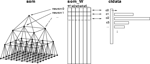
In this section we introduce operations needed for a TS-SOM analysis. First, we give an overview how different data structures are used with TS-SOM. The first operation is training. It builds and organizes a TS-SOM structure, which is stored in the name space with a given name. Suppose that its name is som. In addition, the training creates a weight matrix, which is stored in a data frame called the name of the TS-SOM with the extension _W, for instance, som_W. In that data frame, each data record contains the weights of one neuron, and it is connected to the corresponding neuron through its index. The TS-SOM structure maintains all the structural information about the neural network (see the figure below).
The second important operation is SOM classification. This operation divides the data records of a given data frame into subgroups according to located BMU (neuron). The result is a classified data which includes as many classes as there are neurons in the TS-SOM. Like a weight matrix, one class corresponds to one neuron and includes the indexes of the data records classified to that neuron (see the figure). If the neuron does not get any data record in the classification, then an empty class is created corresponding to that neuron.
| somtr | Train a SOM |
| -d <data> | name of the training data frame |
| -sout <som> | name of TS-SOM structure to be created |
| [-cout <cldata>] | SOM classification to be created |
| [-top] | create the root class |
| [-w <wmat>] | specify a different name for the weight matrix (default <som>_W) |
| [-l <layers>] | the number of layers (default 3) |
| [-md <missing-data>] | a code value to indicate missing data |
| [-D <dimension>] | dimension of the TS-SOM (default 2) |
| [-t <type>] | type of topology (default 0) |
| [-wght <weighting>] | weighting of neighbors (default 0.5) |
| [-c <stop-crit>] | stopping criteria (default 0.001) |
| [-m <max-iter>] | maximum number of iterations (default 20) |
| [-L] | do not use a lookup table (default YES) |
| [-f <corr-layers>] | number of corrected layers (default 3) |
| [-r <train-rule>] | training rule (default 0) |
| partr | Train a SOM using several threads (UNIX/Linux) |
| In addition to somtr: | |
| [-np <threads>] | number of threads to use (default 2) |
The SOM training creates a TS-SOM structure and organizes it. The result includes the structure of the network, stored with the given name <som>. In addition, the weight matrix of TS-SOM is stored in a data frame with the name <som>_W, as described in the figure above. If -cout <cldata> is specified, somtr also creates a classified data frame containing BMU classifications for each data record.
somtr command has lots of parameters, of which the first three are mostly used. Concerning the other parameters, if you are not sure about their use, then you will probably get the best result with their default values. Here are a few parameters described in more detail:
partr is a parallel version of TS-SOM training for UNIX/Linux, and it understands the same switches as the normal single threaded version. In addition, the used may specify the number of threads to use with -np. This number should be a power of 2 (1, 2, 4, 8, 16, ..., 256) and it is inefficient to exceed the number of processors in the used computer.
Example (ex5.1): Training data is created by preprocessing and a SOM is trained using it. In addition, the SOM is used for classification (see command somcl in section 5.1.2).
...
NDA> prepro -d boston -dout predata -e -n
NDA> somtr -d predata -sout som1 -l 4
...
NDA> somcl -d predata -s som1 -cout cld1
| somcl | Classify data by a TS-SOM |
| -s <som> | name of the TS-SOM structure |
| [-w <wmatrix>] | weight matrix, default is to read from <som>_W |
| -d <data> | data to be classified |
| -cout <cldata> | name of the resulting classified data |
| [-md <missing-data>] | a code value to indicate missing data |
| [-top] | create the root class |
This operation classifies data records using a TS-SOM. It creates a classified data in which classes correspond to neurons. Each class has indexes which refer the data records belonging to this class. Note that it is possible to use other weights (or fields) to classify data as were used in the training (see section 5.1.1). To do that, you should select these weights to some data frame, and then give this frame to somcl with the flag -w.
Also, missing data values can be noted. In this case, only such fields that do not include missing values are used to compute the distance between a data record and the neurons of the SOM. See also msdbycen in section 4.1.4 for information about how to replace missing values using the values of the prototypes.
Example (ex5.2): First a TS-SOM is trained using a data frame and then the same data is classified with the same TS-SOM. The second example below uses the result of this example, but loaded from a file.
...
NDA> prepro -d boston -dout predata -e -n
NDA> somtr -d predata -sout som1 -l 4
...
NDA> somcl -d predata -s som1 -cout cld1
# Store trained TS-SOM
NDA> save som1 -o som1
...
Example: This example shows a case, in which a TS-SOM has been trained earlier and stored in a file. The TS-SOM and a data frame are loaded from files, and then the SOM classification is performed. The loaded data is preprocessed first, because the TS-SOM was trained using preprocessed data (see the previous example).
NDA> load som1.som               # name of the TS-SOM is tssom
NDA> load boston.dat             # name of the data is boston
NDA> prepro -d boston -dout preboston
NDA> somcl -d preboston -s som1 -cout cld2
...
| smhsom | Smooth data vectors in neurons |
| -s <som> | name of the TS-SOM structure |
| -d <data> | data to be smoothed |
| -dout <dataout> | name of the resulting data |
| [-hits <hitfield>] | field including hitcounts for clusters |
| [-max <maxit>] | maximum number of iter. (default 50) |
This operation smooths a given data according to the structure of a SOM. Data records corresponding to neurons are averaged by the values of their neighbors. If <hitfield> has been specified, then only empty neurons are recomputed; otherwise updating is performed for all the neurons.
Example (ex5.3): This example shows the effect of smoothing.
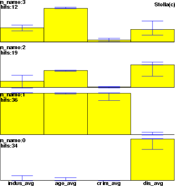
...
NDA> somtr -d pre -sout som -cout cld -l 5
NDA> clstat -d boston -c cld -dout sta -all
NDA> smhsom -s som -d sta -dout smosta -hits sta.hits -max 20
NDA> mkgrp grp1 -s som
NDA> setgdat grp1 -d sta
NDA> layer grp1 -l 4
NDA> bar grp1 -f sta.crim_avg -co red -sca som
NDA> bar grp1 -f sta.chas_avg -co blue -sca som
NDA> mkgrp grp2 -s som
NDA> setgdat grp2 -d smosta
NDA> layer grp2 -l 4
NDA> bar grp2 -f smosta.crim_avg -co red -sca som
NDA> bar grp2 -f smosta.chas_avg -co blue -sca som
| somlayer | Create a field for layer indexes |
| -s <som> | name of the TS-SOM structure |
| -fout <field> | name of the field to be created |
This operation creates a field containing one item per each neuron and fills it with the indexes of TS-SOM layers.
Example (ex5.4): The example shows how layer indexes can be used to pick the weights of one layer. More information about expressions can be found in section 4.4.1.
...
NDA> somtr -d predata -sout som1 -l 5
...
NDA> somlayer -s som1 -fout somlayer
# Select records according to a boolean expression
NDA> selrec -d som1_W -dout l3w -expr 'somlayer' = 3;
| somindex | Store neuron indexes into a frame |
| -s <som> | name of the TS-SOM |
| -dout <data> | data to be created |
This command stores the indexes of neurons into a data frame. The first field will contain the indexes of neurons and other fields (called 0, 1, ...) the coordinates of the neurons. The origin is at the bottom-left corner.
| psl | Pick a SOM layer |
| -s <som> | name of the TS-SOM structure |
| -l <layer> | layer to be dumped |
| -dout <dataout> | data for the SOM grid |
| -wout <wmatrix> | data for the weights of the selected layer |
| [-dim <dimension>] | force the dimension of the data into <dimension> |
| ssl | Set a SOM layer |
| -s <som> | name of the TS-SOM structure |
| -l <layer> | layer index |
| -d <datain> | data to be set |
| -sout <new-som> | new SOM structure |
These commands return or set weights and the SOM grid for a chosen layer. For example, one can use these commands with the Sammon's mapping (see section 5.5).
| calcumat | Compute a U-matrix |
| -s <som> | name of the TS-SOM |
| -d <data> | data for distance computing |
| -umat <umat> | name for the resulting U-matrix data |
| grpumat | U-matrix for groups |
| -s <som> | name of the SOM |
| -w <weights> | prototype data |
| -c <groups> | classified data for the groups |
| -fout <field-out> | resulting field |
| [-in] | within groups, default is between |
This command computes a U-matrix for a TS-SOM. <data> should contain those variables of the neurons, which are used for computing the distances between neurons. The result is a data frame <umat> containing the distance information between neurons. The operation creates a data frame that contains one data record for every neuron. The distances between neurons are stored in fields (2 directions ![]() SOM dimensions). The data frame will be <umat>.data. In addition, the operation stores the minimum and maximum values in each layer in frame <umat>.dminmax. For instructions, how to visualize the U-matrix, see umat (section 8.2.6).
SOM dimensions). The data frame will be <umat>.data. In addition, the operation stores the minimum and maximum values in each layer in frame <umat>.dminmax. For instructions, how to visualize the U-matrix, see umat (section 8.2.6).
grpumat collects U-matrix distances into one field based on specified groups. If flag -in is not given, then distances between neurons of distinct groups are collected, whereas with the flag only distances between the neurons belonging to the same group are picked.
Example: As an example, three weights rm_w, zn_w and age_w are selected to be the basis of distance computing. Then, a U-matrix is computed and created into a graphic structure. To see the result, run the example `ex7.10' (section 8.2.6).
...
NDA> somtr -d boston -sout s1 -l 5
...
NDA> select umatflds -f s1_W.rm_w s1_W.zn_w s1_W.age_w
NDA> calcumat -s s1 -d umatflds -umat umat1
NDA> ls -fr umat1
 umat1.data
 umat1.data.d_0_0
 umat1.data.d_0_1
 umat1.data.d_1_0
 umat1.data.d_1_1
 umat1.dminmax
 umat1.dminmax.min
 umat1.dminmax.max
# Set graphical presentation
NDA> mkgrp grp1 -s s1
NDA> nsize grp1 -v 1.0
NDA> layer grp1 -l 4
NDA> umat grp1 -umat umat1
...
| somsprd | Spread groups |
| -s <som> | name of the TS-SOM |
| -w <prototypes> | data for prototypes |
| -c <core-groups> | the core of the groups |
| -cout <results> | resulting groups |
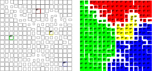
This operation spreads the core groups over the rest of the SOM. New neurons are bound to existing groups from their neighborhood based on the U-matrix distances. The closest neurons are enclosed into a group.
Example: As an example, four neurons have been selected to be the core of the groups. Then, somsprd is used to collect the rest of the neurons to these groups.
...
NDA> somsprd -s som -w som_W -c coreGroups -cout resGroups
...
| somproj | Compute the distances between data records and their BMU neurons |
| -s <som> | name of the TS-SOM structure |
| [-w <wmatrix>] | frame containing the weight matrix |
| -d <data> | data to be classified |
| -c <cldata> | SOM classification |
| -dout <dataout> | name for the resulting data |
This operation computes the distances between data records and their BMU neurons. The operation is executed for each layer of the TS-SOM. The distances are computed in the direction of each SOM dimension, and every dimension of each layer will have its own field, which is named <layer>_<dimension>. The dimensions are indexed starting with zero. The distances are scaled into range [-1,1].
Example (ex5.5): This example shows how distances can be used with trajectories. When the distance data is given to traj (see section 8.2.3), trajectory lines are not drawn between the centroids of the neurons. Instead, the endpoints are moved according to the distances.
NDA> somtr -d pre1 -sout s1 -cout c1 -l 6
...
NDA> somproj -s s1 -w s1_W -d pre1 -c c1 -dout dist1
NDA> clstat -c c1 -d pre1 -dout sta1 -avg -min -max -var -hits
NDA> mkgrp win1 -s s1
NDA> setgdat win1 -d sta1
NDA> setgcld win1 -c c1
NDA> layer win1 -l 4
# Using the mapping with a trajectory
NDA> traj win1 -n a -co red -c c1 -d dist1 -min 0 -max 3000
      -c c1 -d dist1
| somgrid | Generate a data according to the grid of a TS-SOM |
| -s <som> | name of a TS-SOM |
| -min <mindef> | definition for minimum values |
| -max <maxdef> | definition for maximum values |
| -sca <func> | scaling function |
| [-dim <dim>] | index of the SOM's dimension (default 0) |
| [-d <src-data>] | source data for naming |
| [-dout <data-out>] | output data |
| [-fout <field-out>] | output field |
This operation generates new data points according to the grid of a TS-SOM. It creates a data point for each neuron of the given TS-SOM <som>.
The basic idea is to generate values according to the indexes of the neurons. Actually, only one index can run, and it is defined with dimension <dim>. Thus, new values will be constant related to other dimensions. When values are generated, they are scaled into the given range [<mindef>,<maxdef>].
The scaling function <func> defines, how new values are generated. Also, parameters <mindef> and <maxdef> depend on the function as follows:
There are three alternatives, how to name the new data fields. If only one data field is created, then its name can be defined with parameter <field-out>. If parameter <src-data> has been given, then new data fields are named according to fields in this data frame. If both of these parameters have been omitted, new fields are named automatically as f0, f1, ![]()
The data points can be stored in two alternative ways. If the output data frame <data-out> has been specified, then the generated data points are stored there. Otherwise new data fields are added into the current directory.
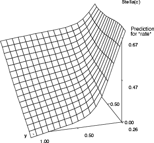
Example (ex5.17): In this example, the MLP network is trained with Boston data (zn, indus ![]() rate). Then, an empty TS-SOM is created for the basis of visualization. Two variables (zn and indus) are used for dimensions x and y by issuing command somgrid, and the trained network is used to predict the value of variable rate for each node of the grid.
rate). Then, an empty TS-SOM is created for the basis of visualization. Two variables (zn and indus) are used for dimensions x and y by issuing command somgrid, and the trained network is used to predict the value of variable rate for each node of the grid.
...
# Train MLP network by the rprop
NDA> select src -f boston.zn boston.indus
NDA> prepro -d src -dout src2 -e
NDA> select trg -f boston.rate
NDA> prepro -d trg -dout trg2 -e
NDA> rprop -d src2 -dout trg2 -net 2 6 1 -full -types t t
      -em 300 -bs 0.01 -mup 1.1 -mdm 0.8 -wout wei -ef virhe
# Build TS-SOM and generate values based on statistics
NDA> somtr build -sout s1 -l 6 -D 2
...
NDA> select x -f src2.zn
NDA> select y -f src2.indus
NDA> fldstat -d x -dout xsta -min -max
NDA> fldstat -d y -dout ysta -min -max
NDA> somgrid -s s1 -min xsta.min -max xsta.max -d x
      -dout datain -sca vec -dim 0
NDA> somgrid -s s1 -min ysta.min -max ysta.max -d y
      -dout datain -sca vec -dim 1
# Predict "rate"
NDA> fbp -d datain -win wei -dout trgout
# Create graphics and show it
NDA> mkgrp /win1 -s /s1
NDA> show win1
The backpropagation algorithm is a supervised learning method for MLP (multi-layer perceptron) networks with sigmoidal activation units. The goal is to find a good mapping from input data to output data. When a new data record is fed to a network, the network provides a good mapping to the output space by using the intrinsic structure of the training set. This implementation allows the user to use several different training methods. Although the basic training algorithm is slow compared to other methods, it can provide, in some cases, a better representation of the training set.
| bp | Create a multi-layer perceptron network using the basic learning rule for training |
| -di <i-data> | name of the input data frame for training |
| -do <o-data> | name of the target data frame for training |
| -net <nlay> <nn1> ... <nnN> | network configuration, number of layers and number of neurons in each layer |
| [-types <s | t | l> ... <s | t | l>] | use a sigmoid, tanh or linear activation function in each layer, default is sigmoid |
| [-ti <ti-data>] | input data frame for test set |
| [-to <to-data>] | target data frame for test set |
| -nout <wdata> | data frame for saving the trained network weights |
| [-vi <vi-data>] | input data frame for a validation set |
| [-vo <vo-data>] | target data frame for a validation set |
| [-ef <edata>] | output error to a frame |
| [-bs <tstep>] | training step length (default is 0.1) |
| [-em <epochs>] | maximum number of training epochs (default is 200) |
| [-one] | forces one neuron / one input |
| [-penalty <penalty>] | regularization coefficient |
The test dataset (-ti, -to) is used as a stopping criterion. The learning does not actually stop, but learning algorithm checks after every successful training epoch, if the error of the test set is smaller than before during the training and saves the network weights. After the maximum number of the training epochs have been reached, these weights are saved to the namespace.
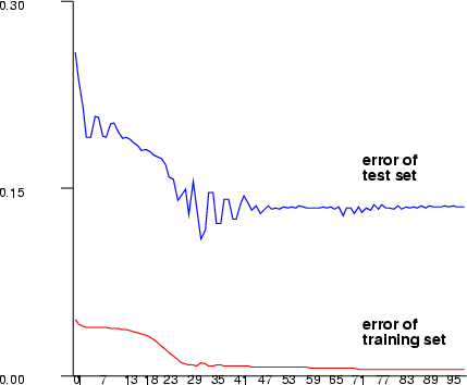
Example (ex5.6): Train a three-layer (input + hidden + output layer) MLP network and save the network output.
NDA> load sin.dat
NDA> select sinx -f sin.x
NDA> select siny -f sin.y
NDA> bp -di sinx -do siny -net 3 1 10 1 -types s s s -em 2000
      -nout wei -ef virhe -bs 0.01
NDA> fbp -d sinx -dout out -win wei
NDA> select output -f sin.x out.0
NDA> save output
| mbp | Create a multi-layer perceptron network using the basic rule with a momentum term for learning |
| -di <i-data> | name of the input data frame for training |
| -do <o-data> | name of the target data frame for training |
| -net <nlay> <nn1> ... <nnN> | network configuration, number of layers, number of neurons in each layer |
| [-types <s | t | l> ... <s | t | l>] | use a sigmoid, tanh or linear network in each layer, default is sigmoid |
| [-ti <ti-data>] | input data frame for test set |
| [-to <to-data>] | target data frame for test set |
| [-vi <vi-data>] | input data frame for a validation set |
| [-vo <vo-data>] | target data frame for a validation set |
| -nout <wdata> | data frame for saving the trained network weights |
| [-ef <edata>] | output error to a frame |
| [-bs <tstep>] | training step length (default is 0.01) |
| [-em <epochs>] | maximum number of training epochs (default is 200) |
| [-mom <moment>] | moment parameter (default is 0.1) |
| [-one] | forces one neuron / one input |
| [-penalty <penalty>] | regularization coefficient |
This command trains an MLP network using the Matlab style training algorithm. The method is based on a global learning rate parameter with a momentum term. By default one neuron for each input is used.
Example (ex5.7): Train a three-layer (input + hidden + output layer) MLP network with sine data using sigmoid activation functions in neurons. After training, save the network output.
NDA> load sin.dat
NDA> select sinx -f sin.x
NDA> select siny -f sin.y
NDA> mbp -di sinx -do siny -net 3 1 10 1 -types s s s -em 1000
      -nout wei -ef virhe -bs 0.2 -mom 0.1
NDA> fbp -d sinx -dout out -win wei
NDA> select output -f sin.x out.0
NDA> save output
| abp | Create a multi-layer perceptron network using a global adaptive training step length |
| -di <i-data> | name of the input data frame for training |
| -do <o-data> | name of the target data frame for training |
| -net <nlay> <nn1> ... <nnN> | network configuration, number of layers, number of neurons in each layer |
| [-types <s | t | l> ... <s | t | l>] | use a sigmoid, tanh or linear network in each layer, default is sigmoid |
| [-ti <ti-data>] | input data frame for test set |
| [-to <to-data>] | target data frame for test set |
| [-vi <vi-data>] | input data frame for a validation set |
| [-vo <vo-data>] | target data frame for a validation set |
| -nout <wdata> | data frame for saving the trained network weights |
| [-ef <edata>] | output error to a frame |
| [-bs <tstep>] | training step length (default is 0.01) |
| [-em <epochs>] | maximum number of training epochs (default is 200) |
| [-mdn <mdown>] | training step multiplier downwards (default is 0.8) |
| [-mup <mup>] | training step multiplier upwards (default is 1.1) |
| [-ac <adapt-cr>] | adaption criterion (default is 1.01) |
| [-one] | forces one neuron / one input |
| [-penalty <penalty>] | regularization coefficient |
This command trains a backpropagation network using a Matlab style training algorithm. This method is based on a global adaptive learning rate parameter. By default one neuron for each input is used.
Example (ex5.8): Train a three-layer (input + hidden + output layer) MLP network with sine data using sigmoid activation functions in the neurons. After training, save the network output.
NDA> load sin.dat
NDA> select sinx -f sin.x
NDA> select siny -f sin.y
NDA> abp -di sinx -do siny -net 3 1 10 1 -types s s s -em 350
      -nout wei -ef virhe -bs 1.2 -ac 1.04 -mup 1.1 -mdn 0.8
NDA> fbp -d sinx -dout out -win wei
NDA> select output -f sin.x out.0
NDA> save output
| mlbp | Create a multi-layer perceptron network using the Matlab neural network toolbox style training |
| -di <i-data> | name of the input data frame for training the network |
| -do <o-data> | name of the target data frame for training the network |
| -net <nlay> <nn1> ... <nnN> | network configuration, number of layers, number of neurons in each layer |
| [-types <s | t | l> ... <s | t | l>] | use a sigmoid, tanh or linear network in each layer, default is sigmoid |
| [-ti <ti-data>] | input data frame for test set |
| [-to <to-data>] | target data frame for test set |
| [-vi <vi-data>] | input data frame for a validation set |
| [-vo <vo-data>] | target data frame for a validation set |
| -nout <wdata> | data frame for saving the trained network weights |
| [-ef <edata>] | output error to a frame |
| [-bs <tstep>] | training step length (default is 0.01) |
| [-em <epochs>] | maximum number of training epochs (default is 200) |
| [-mdm <mdown>] | training step multiplier downwards (default is 0.7) |
| [-mup <mup>] | training step multiplier upwards (default is 1.2) |
| [-mom <moment>] | moment parameter (default is 0.95) |
| [-ac <adapt-cr>] | adapt criterion (default is 1.01) |
| [-one] | forces one neuron / one input |
| [-penalty <penalty>] | regularization coefficient |
This command trains a backpropagation network using the Matlab style of training algorithm. This method is based on a global adaptive learning rate parameter and a momentum term. By default one neuron for each input is used.
Example (ex5.9): Train a three-layer (input + hidden + output layer) MLP network with sine data using sigmoid activation functions in neurons. After training, save the network output.
NDA> load sin.dat
NDA> select sinx -f sin.x
NDA> select siny -f sin.y
NDA> mlbp -di sinx -do siny -net 3 1 15 1 -types t t t -em 100
      -nout wei -ef virhe -bs 0.1 -ac 1.1 -mup 1.1 -mdn 0.7
      -mom 0.95
NDA> fbp -d sinx -dout out -win wei
NDA> select output -f sin.x out.0
NDA> save output
| sabp | Create a multi-layer perceptron network using the Silva & Almeida training |
| -di <i-data> | name of the input data frame for training the network |
| -do <o-data> | name of the target data frame for training the network |
| -net <nlay> <nn1> ... <nnN> | network configuration, number of layers, number of neurons in each layer |
| [-types <s | t | l> ... <s | t | l>] | use a sigmoid, tanh or linear network in each layer, default is sigmoid |
| [-ti <ti-data>] | input data frame for test set |
| [-to <to-data>] | output data frame for test set |
| [-vi <vi-data>] | input data frame for a validation set |
| [-vo <vo-data>] | target data frame for a validation set |
| -nout <wdata> | data frame for saving the trained network weights |
| [-ef <edata>] | output error to a frame |
| [-bs <tstep>] | training step length (default is 0.01) |
| [-em <epochs>] | maximum number of training epochs (default is 200) |
| [-mdm <mdown>] | training step multiplier downwards (default is 0.8) |
| [-mup <mup>] | training step multiplier upwards (default is 1.1) |
| [-one] | forces one neuron / one input |
| [-penalty <penalty>] | regularization coefficient |
This command trains an MLP network using the Silva & Almeida training algorithm. This method is based on adaptive learning rate parameters on each neuron's weight. Unlike in the RPROP algorithm the maximum and minimum learning rate is not defined in this algorithm. By default, one neuron for each input is used.
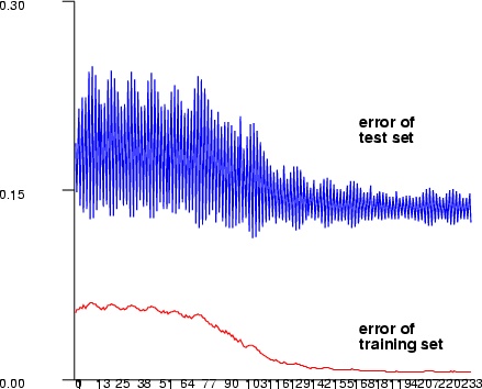
Example (ex5.10): Train a three-layer (input + hidden + output layer) MLP network with sine data using sigmoid activation functions in neurons. After training, save the network output and plot the training error graph.
NDA> load sin.dat
NDA> select sinx -f sin.x
NDA> select siny -f sin.y
NDA> sabp -di sinx -do siny -net 3 1 10 1 -types s s s -em 100
      -nout wei -ef virhe -bs 1.0 -mup 1.1 -mdm 0.8
NDA> fbp -d sinx -dout out -win wei
NDA> select train -f virhe.TrainError
NDA> select output -f sin.x out.0
NDA> save output
NDA> mkgrp xxx
NDA> ldgrv xxx -f virhe.TrainError -co black
NDA> show xxx
| rprop | Create a multi-layer perceptron network using the RPROP training |
| -di <i-data> | name of the input data frame for training the network |
| -do <o-data> | name of the target data frame for training the network |
| -net <nlay> <nn1> ... <nnN> | network configuration, number of layers, number of neurons in each layer |
| [-types <s | t | l> ... <s | t | l>] | use a sigmoid, tanh or linear network in each layer, default is sigmoid |
| [-ti <ti-data>] | input data frame for test set |
| [-to <to-data>] | output data frame for test set |
| [-vi <vi-data>] | input data frame for a validation set |
| [-vo <vo-data>] | target data frame for a validation set |
| -nout <wdata> | data frame for saving the trained network weights |
| [-ef <edata>] | output error to a frame |
| [-bs <tstep>] | training step length (default is 0.01) |
| [-em <epochs>] | maximum number of training epochs (default is 200) |
| [-mdm <mdown>] | training step multiplier downwards (default is 0.8) |
| [-mup <mup>] | training step multiplier upwards (default is 1.1) |
| [-smin <min-tsl>] | minimum training step length (default is 0.0001) |
| [-smax <max-tsl>] | maximum training step length (default is 10.0) |
| [-one] | forces one neuron / one input |
| [-penalty <penalty>] | regularization coefficient |
This command trains a backpropagation network using the RPROP training algorithm. The method is based on adaptive learning rate parameters on each neuron's weight. By default, one neuron for each input is used.
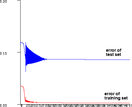
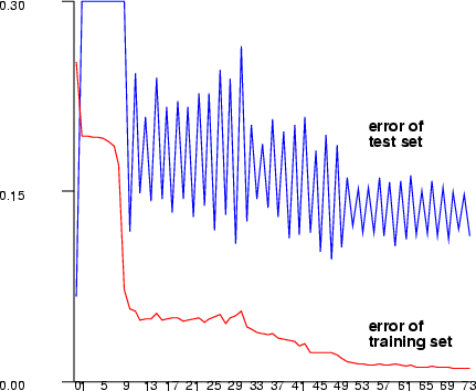
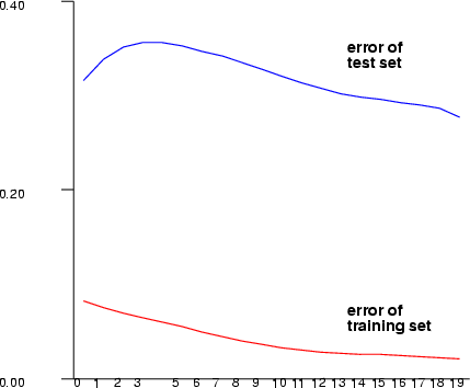
Example (ex5.11): Train a three-layer (input + hidden + output layer) MLP network with sine data using sigmoid activation functions in neurons. After training is done, save the network output and error.
NDA> load sink.dat
NDA> load sint.dat
NDA> select sinx -f sink.ox
NDA> select siny -f sink.oy
NDA> select sinox -f sink.ox
NDA> select sintx -f sint.tx
NDA> select sinty -f sint.ty
NDA> rprop -di sinx -do siny -net 3 1 3 1 -types s s s -em 40
      -bs 0.05 -mup 1.1 -mdm  0.8 -nout wei -ti sintx -to sinty
      -ef virhe
NDA> fbp -d sinox -dout out -win wei
NDA> select test -f virhe.TrainError virhe.TestError
NDA> select output -f sink.ox out.0
NDA> save output
NDA> save test
| lmbp | Create a multi-layer perceptron network using the Levenberg-Marquard training |
| -di <i-data> | name of the input data frame for training the network |
| -do <o-data> | name of the target data frame for training the network |
| -net <nlay> <nn1> ... <nnN> | network configuration, number of layers, number of neurons in each layer |
| [-types <s | t | l> ... <s | t | l>] | use a sigmoid, tanh or linear network in each layer, default is sigmoid |
| [-ti <ti-data>] | input data frame for a test set |
| [-to <to-data>] | target data frame for a test set |
| [-vi <vi-data>] | input data frame for a validation set |
| [-vo <vo-data>] | target data frame for a validation set |
| -nout <wdata> | data frame for saving the trained network weights |
| [-ef <edata>] | output error to a frame |
| [-lamda <lamda>] | regularization parameter for controlling the step size (default is 1.0) |
| [-mdm <mdown>] | regularization parameter multiplier downwards (default is 1.1) |
| [-mup <mup>] | regularization parameter multiplier upwards (default is 0.9) |
| [-one] | forces one neuron / one input |
| [-penalty <penalty>] | regularization coefficient |
This command trains a backpropagation network using the Levenberg-Marquard training algorithm. This method is based on approximating the second order derivatives by using the first order derivatives. The method is quite sensitive to its regularization parameters. By default, one neuron for each input is used.
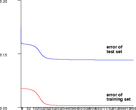
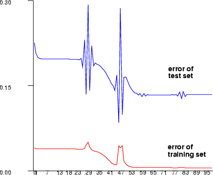
Example (ex5.12): Train a three-layer (input + hidden + output layer) MLP network with sine data using sigmoid activation functions in neurons. After training is complete, print the training and testing error graphs.
NDA> load sint.dat
NDA> load sink.dat
NDA> select sinx -f sink.ox
NDA> select siny -f sink.oy
NDA> select sinox -f sink.ox
NDA> select sintx -f sint.tx
NDA> select sinty -f sint.ty
NDA> lmbp -di sinx -do siny -net 2 3 1 -types s s s -nout wei
      -ef virhe -lamda 1.0 -mup 2.0 -mdn 0.8 -em 40
      -ti sintx -to sinty
NDA> fbp -d sinox -dout out -win wei
NDA> mkgrp xxx
NDA> ldgrv xxx -f virhe.TrainError -co black
NDA> ldgrv xxx -f virhe.TestError -co red
NDA> show xxx
| fbp | Use a trained network |
| -d -dout <dataout> | name of the output data frame for network mapping |
| -nin <wdata> | input data frame for the trained network weights |
| [-layer <layer>] | make output data from network layer <layer> |
This command uses a trained network. For the use see the previous examples and the example below. One remark of using -layer option: user should keep in mind that the layer numbers start from zero.
In order to explore the trained MLP network, one can use the TS-SOM structure. The basic idea is to generate an artificial data space for inputs such that each neuron of the TS-SOM is set to some point of this data space. Then, the trained MLP network is used to compute output values for the generated points. The TS-SOM structure can then be used to present data points in the input and output spaces. See also the example ex5.18.
In the following example, the MLP network is trained with Boston data to obtain relationships between some background variables and the prices of the appartments. Then, new values of these background variables are generated and the output values are computed by the trained network to each neuron of the TS-SOM.
First, the MLP network is trained as follows:
NDA> load boston.dat
NDA> select inputflds -f boston.crim boston.zn boston.ptratio
      boston.b boston.chas boston.dis boston.indus
NDA> select trg -f boston.rate
NDA> prepro -d trg -dout trg2 -e
NDA> prop -di src2 -do trg2 -net 2 15 1 -types s s -em 300
      -bs 0.01 -mup 1.1 -mdm 0.8 -nout wei -ef virhe
The following commands show an example how the input and output data of the MLP network can be visualized. An empty TS-SOM structure is created and then data points are generated for each neuron to represent one point in the input space (see somgrid in section 5.1.10). In the first example, field crim will increase according to the x-coordinates and the field zn according to the y-coordinates of the neurons. The rest of the fields (ptratio, b, chas, dis and indus) are kept as constant values that are their averages.
NDA> select x -f inputflds.crim
NDA> select y -f inputflds.zn
NDA> select z -f inputflds.ptratio inputflds.b inputflds.chas
      inputflds.dis inputflds.indus
NDA> fldstat -d x -dout xsta -min -max
NDA> fldstat -d y -dout ysta -min -max
NDA> fldstat -d z -dout zsta -avg
# Create an empty TS-SOM and generate data points for its neurons
NDA> somtr build -sout s1 -l 6 -D 2
...
NDA> somgrid -s s1 -min xsta.min -max xsta.max -d x -dout x1
      -sca vec -dim 0
NDA> somgrid -s s1 -min ysta.min -max ysta.max -d y -dout y1
      -sca vec -dim 1
NDA> somgrid -s s1 -min zsta.avg -max zsta.avg -d z -dout z1
      -sca vec -dim 0
# Compute output values by the MLP network
NDA> select data1 -f x1.crim y1.zn z1.ptratio z1.b z1.chas
      z1.dis z1.indus
NDA> fbp -d data1 -nin wei -dout trgout
NDA> select data1 -d trgout
NDA> mkgrp win1 -s /crim_zn/s1
NDA> setgdat win1 -d /crim_zn/data1
...
NDA> ngray /crim_zn/win1 -f /crim_zn/data1.0 -sca som
NDA> bar /crim_zn/win1 -inx 0 -f /crim_zn/data1.zn -co green
NDA> bar /crim_zn/win1 -inx 1 -f /crim_zn/data1.crim -co red
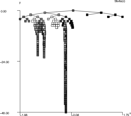
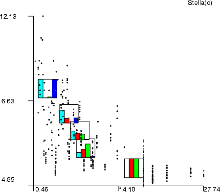
By using similar command sequences, we can visualize the relationships between different combinations of the background variables and outputs of the MLP network. The results are presented below.
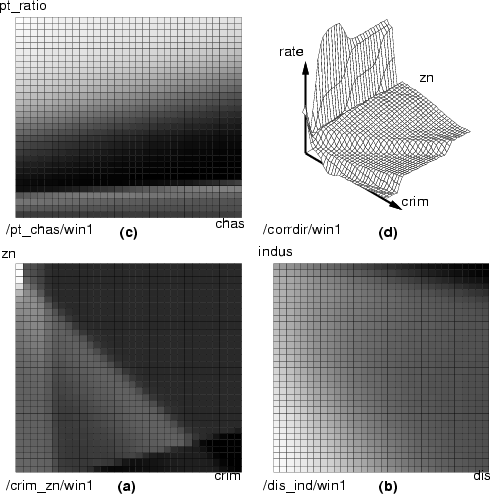
In the three grayscale figures the gray level of the boxes describes the output values and two background variables are mapped to the x and y axes. In the last figure, the output is mapped to the z axis. Figure a) the background variables are crim and zn; figure b) the background variables are ptratio and chas; figure c) the background variables are dis and indus. In figure d) the variables crim, b and indus increase on the x-axis and the variables zn, chas and dis increase on the y-axis. The predicted variable rate is mapped to the z-axis. Note that the last example also uses other background variables for computing, but only these two have been displayed.
This special command allows you to search for such input values for an MLP neural network that correspond to given outputs.
| inputsearch | Searching for MLP-inputs |
| -n <mlp> | the frame with MLP weights |
| -d <pretarget> | the data frame with desirable (preprocessed) outputs |
| -dout <result> | the name of the result data frame |
| [-p <points>] | the number of starting points (default 1) |
| [-it <iterations>] | the number of iterations (default is 1000) |
| [-fac <factor>] | the factor's values (default is 0.7) |
Assume that the studied phenomenon concerns the number of outputs
![]() and inputs
and inputs
![]() . Then, an MLP neural network is trained to model this phenomenon. In other words, the network is used to estimate values
. Then, an MLP neural network is trained to model this phenomenon. In other words, the network is used to estimate values ![]() by values of
by values of ![]() . Often it is useful to solve the inverse problem; to find out the input values that give us certain output values. The inputsearch command can be used to obtain these input values using an algorithm similar to the Gibbs sampler.
. Often it is useful to solve the inverse problem; to find out the input values that give us certain output values. The inputsearch command can be used to obtain these input values using an algorithm similar to the Gibbs sampler.
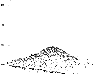
The idea of the algorithm is as follows. A random walk along the estimated MLP surface is conducted by advancing from a random starting point by randomly changing the value of one input parameter at a time. The main goal is to locate the points in the input parameter space, which give the desired output values. The rule of the random walk is to accept always the next point if its goodness is better than the goodness of the previous point, and to accept it with a probability that depends on the difference between points' goodnesses, if the goodness of the next point is worse. The bigger the difference the smaller the probability to move to the next point. If the point is rejected another point is taken. While walking the point whose output values are closest to the desired values is stored. Parameters for the command are: -n specifies the data frame with weights of the trained MLP, -d the data frame with desirable outputs, preprocessed with the same statistics as used for preprocessing of the outputs in the MLP training process, and -dout the name of the data frame with results.
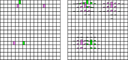
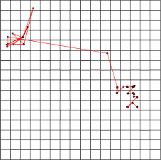
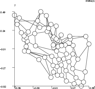
Assume that the MLP has been trained to model a normal bivariate function (see the first figure below). The inputs for the MLP are parameters ![]() and
and ![]() , and the output is
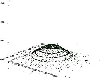
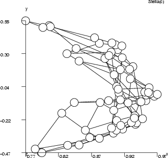
, and the output is ![]() , and the goal is to find those input combinations that give us the output value 0.2. It is obvious that there are many such combinations and they form some kind of curve in the 3-D space. The inputsearch algorithm will find one combination of inputs for each starting point, so a large number of starting points is needed in order to obtain several point from the curve. The number of starting points should in most cases be 100 or more (parameter -p). The second figure below illustrates the results of input searching for the output values 0.2, 0.3, 0.4 and 0.5, with 200 starting points for each search.
, and the goal is to find those input combinations that give us the output value 0.2. It is obvious that there are many such combinations and they form some kind of curve in the 3-D space. The inputsearch algorithm will find one combination of inputs for each starting point, so a large number of starting points is needed in order to obtain several point from the curve. The number of starting points should in most cases be 100 or more (parameter -p). The second figure below illustrates the results of input searching for the output values 0.2, 0.3, 0.4 and 0.5, with 200 starting points for each search.
Switch -it specifies the number of iterations or steps the algorithm should accomplish. The higher the number of steps the better the accuracy of the results. However, a large number of steps increases the amount of computing time required. The number of iterations should be 10000, or more.
Switch -fac specifies a value, which influences the length of the steps. By default the value is 0.7, and it can be adjusted between 0 and 1. In the algorithm a point, whose goodness is worse than the goodness of the previous point can be accepted with a probability, which depends on the difference between the goodnesses of those points. If the difference is large a longer step is taken from this point in order to move away from the bad region of the surface. In this case the value specified with switch -fac controls the size of this step.
Example: This example script demonstrates the use of inputsearch.
# Generating bivariate function
gen -N 0.5 0.5 -dout gauss -s 1000 -dim 2

# Calculating outputs
expr -fout gauss.out -expr (1/sqrt(2*3.141592*0.5))\
  *(exp(-( ('gauss.F0'-0.5)^2-('gauss.F1'-0.5)^2 )/(2*0.5) ) );

select input -f gauss.F0 gauss.F1
select output -f gauss.out

# Calculating statistics
fldstat -d output -dout stat -min -max
fldstat -d input -dout stat2 -min -max

# Preprocessing data
prepro -d input -dout preinput -e
prepro -d output -dout preoutput -e

# Training the MLP neural network
rprop -di preinput -do preoutput -net 3 2 25 1\
  -types s s s -nout wei -em 1000 -bs 0.002

# Desired output
expr -fout wanted -expr 0.4;
select desire -f wanted

# Preprocessing according to previous statistics
prepro -d desire -dout predesire -d2 stat -e

@echo Start searching
inputsearch -n wei -d predesire -dout data\
         -p 200 -it 10000 -fac 0.7

# Calculating values in original scale
expr -dout result -fout par1  -expr\
  'data.input1'*(${stat2.max[0]}-${stat2.min[0]})+${stat2.min[0]};
expr -dout result -fout par2  -expr\
  'data.input2'*(${stat2.max[1]}-${stat2.min[1]})+${stat2.min[1]};
expr -dout result -fout opt -expr\
  'data.output1'*(${stat.max[0]}-${stat.min[0]})+${stat.min[0]};

# Saving results
save result

# Visualizing results
mkgrp picture
axis picture -ax z -sca abs -min 0.0 -max 2.0 -step 4
axis picture -ax x -sca abs -min -1.0 -max 2.0 -step 10
axis picture -ax y -sca abs -min -1.0 -max 2.0 -step 10

# Plotting the original bivariate function
datplc picture -n gauss -ax x -f gauss.F0 -co green
datplc picture -n gauss -ax y -f gauss.F1 -co green
datplc picture -n gauss -ax z -f gauss.out -co green

# Plotting points with output value 0.4
datplc picture -n r -ax x -f result.par1 -co black
datplc picture -n r -ax y -f result.par2 -co black
datplc picture -n r -ax z -f result.opt -co black

viewp picture -dz 150 -dy 0 -xy 42 -yz -70
show picture
This is an alternative MLP implementation, which is based on derivatives.
| mlp2layer | Stochastic learning |
| -di <output> | name of frame with inputs |
| -do <input> | name of frame with outputs |
| -hi <nn> | number of neurons in hidden layer |
| -t1 <s|t|l> | activation function in the hidden layer |
| -t2 <s|t|l> | activation function in the output layer |
| -wout <weight> | frame with network weights |
| [-err <error>] | frame with errors |
| [-iter <NN>] | number of iterations, default 10000 |
| [-reg <regular>] | regularization term, default 0.0 |
| -batch | use batch learning |
NDA> load data.dat
NDA> select inputs -f data.x1 data.x2
NDA> select outputs -f data.y1 data.y2
NDA> prepro -d inputs -dout prein -e
NDA> prepro -d outputs -dout preout -e
NDA> mlp2layer -di prein -do preout -hi 5 -t1 s -t2 s wout weights \
     -err errors -iter 1000000 -reg 0.001
| mlp2layer | MLP using Rprop learning |
| -di <output> | name of frame with inputs |
| -do <input> | name of frame with outputs |
| -hi <nn> | number of neurons in hidden layer |
| -t1 <s|t|l> | activation function in the hidden layer |
| -t2 <s|t|l> | activation function in the output layer |
| -wout <weight> | frame with network weights |
| [-hess <hessian>] | frame with the hessian matrix |
| [-err <error>] | frame with errors |
| [-iter <NN>] | number of iterations, default 10000 |
| [-reg <regular>] | regularization term, default 0.0 |
| -rprop | use rprop learning |
| [-min <min>] | step size control minimum, default 0.000001 |
| [-max <max>] | step size control maximum, default 10 |
| [-inc <inc>] | multiplier upwards, default 1.1 |
| [-dec <dec>] | multiplier downwards, default 0.8 |
NDA> load data.dat
NDA> select inputs -f data.x1 data.x2
NDA> select outputs -f data.y1 data.y2
NDA> prepro -d inputs -dout prein -e
NDA> prepro -d outputs -dout preout -e
NDA> mlp2layer -di prein -do preout -hi 5 -t1 s -t2 s wout weights \
    -err errors -iter 200 -reg 0.001 -rprop -hess hessian
| mlpout | Network outputs calculation |
| -d <inputs> | name of frame with inputs |
| -dout <outputs> | name of frame with outputs |
| -nin <weights> | name of frame with mlp weights |
| [-sens <sensitivity>] | prefix for the sensitivity matrices |
| [-ggt <GGT>] | frame with GGT matrix |
| [-cov <covariance>] | frame with covariance matrix |
| [-jacob <jacobian>] | frame with jacobian matrix |
The function mlpout calculates the MLP-neural networks outputs for the given inputs. If the prefix with the switch -sens is given then the function will calculate the outputs sensitivity matrix. Which contain the values
![]() , where
, where ![]() is the network output, and
is the network output, and ![]() is the weight of the network. The sensitivity matrixes are calculated for each input record. Thus, there will be as many frames with the sensitivity matrix as there are records in the input frame.
is the weight of the network. The sensitivity matrixes are calculated for each input record. Thus, there will be as many frames with the sensitivity matrix as there are records in the input frame.
The switch -ggt is useful when we want to calculated the approximation of the Fisher Information Matrix for the MLP neural network, that is the quantity
![]() , where the summation will be done over all inputs. Note that in this case the inputs given with the -d must be the same as ones used for the MLP network training procedure. Also the user must point the covariance matrix
, where the summation will be done over all inputs. Note that in this case the inputs given with the -d must be the same as ones used for the MLP network training procedure. Also the user must point the covariance matrix
![]() with the -cov switch. It can be for example covariance of residuals of the MLP outputs.
with the -cov switch. It can be for example covariance of residuals of the MLP outputs.
Further, the Jacobian matrixes for every inputs can be calculated if the prefix -jacob is given. Each matrix will contain the values
![]() , where
, where ![]() is the network output, and
is the network output, and ![]() is the input.
is the input.
| classical | Scale a data set from a greater to a lower dimension by using the PCA (Principal Component Analysis) |
| -d <data> | name of the input data frame |
| -dout <dataout> | name of the output data frame |
| -dim <dim> | dimension for the output data |
| [-pcout <pcdata>] | saves eigenvalues and eigenvectors of covariance matrix |
| sammon | Scale data from a greater to a lower dimension by using the Sammon's mapping |
| -d <data> | name of the input data frame |
| -dout <dataout> | name of the output data frame |
| -dim <dim> | dimension for output data (default 2) |
| [-eps <stop>] | stopping criterion (default 0.0) |
| [-ef <efile>] | write error in every iteration to a file and window |
| [-imax <imax>] | maximum iteration steps (default 30) |
| [-dinit <inidata>] | initial values for the output data |
These multidimensional scaling commands seek to preserve some notions of the geometric structure of the original data, while reducing dimensionality. The points, which lie close to each other in the input space will appear similarly close in the output space. These two commands use different methods for preserving the intrinsic structure of the data. Classical scaling tries to map data points in an optimal fashion to the output space by using a principal component analysis. The Sammon's mapping maps data points to the output space by minimizing the distance difference between data points in the input and output spaces.
Example (ex5.13): The Sammon's mapping and classical scaling.
...
NDA> prepro -d boston -dout preboston -e -n
NDA> somtr -d preboston -sout somboston -l 5 -cout cluboston
...
# Pick weights
NDA> psl -s somboston -dout grid3 -l 3 -wout w3
# Sammon mapping
NDA> sammon -dinit grid3 -d w3 -dout out3 -imax 30 -eps 0.01
      -ef virhe
# Setting transformed values for SOM
NDA> ssl -s somboston -sset out3 -sout trans -l 3
# The same for the classical scaling
NDA> classical -d w3 -dout class_out -dim 2
NDA> ssl -s somboston -sset class_out -sout class_weights -l 3
...
This command makes a principal component analysis for a data set. Principal component analysis (PCA) is a mathematical procedure, which transforms a number of (possibly) correlated variables into a (smaller) number of uncorrelated variables called principal components. The first principal component accounts for as much of the variability in the data as possible, and each succeeding component accounts for as much of the remaining variability as possible. The objectives of principal component analysis are: to discover or to reduce the dimensionality of the data set, and to identify new meaningful underlying variables.
| principal | Principal component analysis |
| -d <data_in> | name of the data frame to be analyzed |
| -dout <data_out> | name of the data frame with new coordinates of points |
| [-cov <covariance>] | covariance matrix of data (optional) |
| [-e <eigen>] | name for the data frame with eigenvalues and eigenvectors (default is eigen) |
The command requires the name of the data frame and a name for the output frame where the new coordinates of the data points will be stored. The covariance matrix of the data can be calculated in beforehand. However, if the name of the covariance matrix is not specified the function will calculate this matrix by itself. The eigenvalues and eigenvectors will be stored in the data frame specified with -e (by default it will be a data frame called eigen).
Example: Here is an example script of the use of principal.
NDA>principal -d data_in -dout new_coord
NDA>ls -fr new_coord
new_coord.f_1
new_coord.f_2
new_coord.f_3
new_coord.f_4
NDA>ls -fr eigen
eigen.value
eigen.vec_1
eigen.vec_2
eigen.vec_3
eigen.vec_4
This command fits a linear regression model to the data set, and calculates confidence and prediction bands for the regression.
| confbands | Linear regression and confidence bands |
| -f <output> | name of the field with response values ( |
| -d <input> | name of the data frame with factors input data |
| -d2 <points> | name of the frame with data points for which confidence bands will be calculated |
| -conf <level> | value of the confidence level |
| -fout <coeff> | name for the field where the coefficients of the regression model will be stored |
| -dout <bands> | name for the data frame where confidence and prediction bands will be stored |
The most typical type of regression is linear regression (meaning the use of a straight line for fitting in a two dimensional case, rather than some other type of curve) constructed using the least-squares method (the chosen line is the one that minimizes the sum of the squares of the distances between the line and the data points).
In a multi-dimensional space the linear regression model can be represeted as
![]() , where
, where ![]() is the respose factor which depends on input variables
is the respose factor which depends on input variables
![]() and some coefficients
and some coefficients
![]() . Thus, the confbands function calculates the coefficients of the regression model and stores them into the output field <coeff>. The length of the field <output> and the length of the fields in the data frame <input> must be the same.
. Thus, the confbands function calculates the coefficients of the regression model and stores them into the output field <coeff>. The length of the field <output> and the length of the fields in the data frame <input> must be the same.
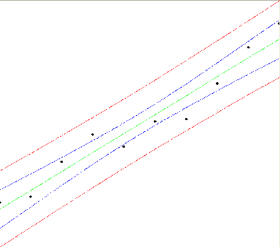
In order to calculate the confidence and prediction bands for the regression model the command requires a data frame specifying the points in which those bands are to be calculated (switch -d2). Using switch -conf the confidence level can be specified. This value must be between 0 and 1. The command stores the confidence and prediction bands into the data frame named with -dout. Five fields will be created: up_pred and low_pred contain the values of the upper and lower prediction bands in the points given in data frame <points>, up_conf and low_conf contain the values of the upper and lower confidence bands, and regression contains the values of the regression fit.
Example: Here is an example of fitting a straight line into a two dimensional data set.
#### data ####
x       y       |     x       y
1.0     2.0     |     6.0     8.8
2.0     2.5     |     7.0     9.0
3.0     5.4     |     8.0    12.0
4.0     7.7     |     9.0    15.0
5.0     6.7     |    10.0    17.0
##############

NDA> ls -fr data
data.x
data.y
select input -f data.x
select points -f data.x
NDA> confbands -f data.y -d input -d2 points -conf 0.95 \
      -fout coeff -dout bands
NDA> getdata coeff
2
-0.106667
1.584849
A visualization of the confidence (blue) and prediction (red) bands for the regression (green) is given in the following picture.
The NDA kernel includes some basic clustering algorithms that are introduced in this chapter.
| hclust | Hierarchical clustering |
| -sl | single link clustering (MERGE) |
| -al | average link clustering (MERGE) |
| -cl | complete link clustering (MERGE) |
| -ce | centroid (group average) (MERGE) |
| -me | median clustering (MERGE) |
| -mv | min variance clustering (MERGE) |
| -2m | 2-means clustering (SPLIT) |
| -ms | Macnaughton-Smith clustering (SPLIT) |
| -d <datain> | the name of the input data frame |
| -dout <dataout> | the name of the output data frame |
| -cout <cldata> | data frame for clusters |
| -clvis <clvis> | data frame for tree structures in visualization |
| [-cut <layer>] | choose in which layer to cut the tree |
| [-verbose ] | request additional information about the clustering process |
This operation divides the data set, <data>, into clusters by hierarchical clustering algorithms. The centroids of the clusters are stored into the frame <dataout> and classification of data records into <cldata>. The flag -clvis is used for visualization. The frame <clvis> contains the tree structure of the network. Please note, that the visualization tree structure does not visualize the locations of the actual clusters of data!
Example (ex5.14): This example shows the basic use of the command.
NDA> load boston.dat
NDA> select cluflds -f boston.indus boston.crim boston.zn
      boston.rate
NDA> hclust -d cluflds -dout hcludat -cout cld -clvis hhier -sl
NDA> mkgrp win1 -d hcludat
NDA> setgdat win1 -d hcludat
NDA> topo win1 -c hhier -on
...
| kmeans | k-means clustering |
| -d <data> | name of the input data frame |
| -dout <dataout> | name of the output data frame |
| -cout <cldata> | data frame for clusters |
| -k <k> | number of k-means clusters |
This command performs the k-means clustering algorithm in order to divide data into <k> clusters. The centroids of the clusters are stored into the frame <dataout> and the classification information of data records into the classified data <cldata>.
Example (ex5.15): In the example, the Boston data is divided into five clusters, which are visualized through their centroids.
NDA> load boston.dat
NDA> select flds -f boston.indus boston.age boston.zn boston.dis
NDA> kmeans -d flds -dout clusdat -cout cluscld -k 5
NDA> mkgrp win1 -d clusdat
...
| fcm | Fuzzy c-means clustering algorithm |
| -d <data> | name of the input data frame |
| -dout <dataout> | output data frame |
| -cout <cldata> | cluster frame |
| -eps <s-float> | stopping criterion |
| -imax <int> | maximum number of iterations |
| -nclu <nclust> | number of clusters/prototypes |
| [-my <c-float>] | clustering criterion |
This command executes the fuzzy c-means algorithm in order to divide the data set, <data>, into clusters. The centroids of the clusters are stored into data frame <dataout> and the classification information to the classified data <cldata>. The number of clusters is defined with the flag -nclu. If no clustering criterion is given put inputdata to nearest cluster.
Example (ex5.16): This example demonstrates the basic use of fcm.
NDA> load boston.dat
NDA> select flds -f boston.indus boston.dis boston.crim boston.age
NDA> fcm -d flds -dout clusdat -cout clucld -eps 0.0 -fi 3
      -my 0.7 -nclu 4 -imax 100
...