Image processing

There are three different image types: grayscale, indexed color and true color. Grayscale is an 8 bit gray-level picture without a colormap. Indexed color is also 8 bit, but contains an RGB colormap. True color represents each pixel with 24 bits containing 8 bits for all three color components: red, green and blue.

File commands

Used for loading and saving of G(raphics)I(nterchange)F(ormat) image files.

loadimg	Load a GIF image file into memory
<filename>	GIF file name
[<dataname>]	image name for name space (default is <filename> without the extension)

This command loads a GIF file into the name space.

saveimg	Save an image into a GIF file
<dataname>	image name in name space
[<filename>]	file to be written (default is to use <dataname> with extension .gif)

This command writes an image structure into a GIF file. Original image needs to be of type indexed color.

Image conversions and cropping

cnvimg	Convert an image into some other format
-in <input>	source image
-out <output>	destination image
-gray |	convert source into a grayscale image
-indc |	convert source into indexed color
-true	convert source into a true color image

This command attempts to convert some image into another format as well as possible.

crop	Crop an area out of an image
-in <image>	source image
-out <imgout>	destination image
-x0 <x-coord>	the x-coordinate of the starting corner
-y0 <y-coord>	the y-coordinate of the starting corner
-w <w>	the width of the cropping
-h <h>	the height of the cropping

This command crops an area out of the image for later processing.

convmatrix	Convert a given image into matrix presentation
-in <image>	image to convert
-out <matrix>	resulting matrix
[-sign]	if given, the image is thought to consist of signed numbers

This command converts a given image into matrix presentation (see section 2.17.1 for further details).

Example (ex6.1):

NDA> loadimg i003.gif pict1
# Masking 
NDA> matrix mask.real [0, -1, 0; -1, 4, -1; 0, -1, 0]
# Grayscale - pictures 
NDA> cnvimg -in pict1 -out pict -gray
# Convert image to matrix
NDA> convmatrix -in pict -out matrix
...

Conversions between images and data frames

f2i	Convert a data frame into an image
-d <frame>	input frame name.
-iout <image>	output image name.
[-verbose]	output extra info during conversion
[-bgimg <bgimage>]	background image
[-bgcol <gray | r g b>]	background gray level or rgb color
[-xsize <x>]	horizontal dimension for output image
[-ysize <y>]	vertical dimension for output image
i2f	Convert an image into a data frame
-i <image>	input image name
-dout <frame>	output frame name
[-gray]	convert color image to grayscale
[-rgb]	convert grayscale image to indexed

Command f2i converts a frame into an image. The frame must contain three fields. The first field is used for the x coordinate, second for the y coordinate and third for the grayscale level of the pixels. If there exists five fields then the last three fields are used as RGB values for the image and a palette is created before converting the frame into an image. The option -verbose provides the user extra information while converting the frame into an indexed image. If there are less pixels in the input data frame than in the output image, other pixels are specified by background image and background color. Size of output image is based on background image and given pixels if size is not specified explicitly using -xsize and -ysize.

Command i2f converts an image into a data frame. If the input image is grayscale then the output frame contains three fields x, y and img, where fields x and y are the corresponding coordinates of pixel value img. The field img contains the gray value of the pixel. When using option -rgb the frame contains fields x, y, red, green, blue, which contain the coordinates and RGB values of the pixels. If the input image is indexed, the output frame contains five fields x, y, red, green, blue, unless option -gray is used, in which case the image is converted into a grayscale image before making the conversion to a frame.

Example: This simple example reads a grayscale image gray.gif into namespace and then converts it into a data frame and back again into an image.

NDA> loadimg gray.gif
NDA> i2f -i gray -dout imgframe
# Save the frame to disk
NDA> save imgframe
...
# After some operations convert the result back to an image
NDA> f2i -d newimgfrm -iout newgray

Converting graphs into pixel data frames

gr2fr	Convert graph into data frame
-vdata <nodes>	graph nodes
-edata <arcs>	graph arcs
-dout <pixeldata>	data frame containing pixels

This command converts a graph into data frame that contains pixels and colors for plotting the graph using f2i command. A graph structure is defined using two data frames, <nodes> and <arcs>. Data frame <nodes> contains at least three fields having type int or float. First field is considered as horizontal coordinate, second vertical coordinate and third gray level. Other fields may contain some other node related information and are ignored. Data frame <arcs> contain at least two fields. They must have type int. First field is considered as begin node index (first index is zero) and second field end node index of an arc. Other fields may contain some other arc related information and are ignored.

Example: Assuming that nodes and arcs define a graph, following commands plot the graph.

...
# Convert graph into pixels
NDA> gr2fr -vdata nodes -edata arcs -dout pix
# Convert pixels into image
NDA> f2i -d pix -iout img -bgcol 0 -xsize 256 -ysize 256
Doing grayscale
Image is 256 x 256.
# Show image
NDA> mkgrp g
NDA> bgimg g -img img
NDA> show g

Creating an image mosaic according to a SOM

mosaic	Create an image mosaic according to a SOM
-out <image>	image to be created
-c <cldata>	classified data frame for the mosaic (SOM classification)
-f <namfld>	a field containing image file names in the O/S filesystem
-l <layer>	SOM layer to be used for mosaic ($2^{2 layer}$ images will be presented
-w <width>	width of the image to be created
-h <height>	height of the image to be created
-frame <fw>	width for the frame that separates the images
[-corner]	take a crop from the top left corner of the image instead of sampling the whole image

This command creates an image mosaic according to a SOM classification. The subimages of the mosaic are read from the O/S filesystem using <namfld> for the filenames. The size of the mosaic can be specified with <width> and <height>, and a border of <fw> pixels is drawn around each image. The size of each component image is reduced by taking the top left corner or by sampling the whole image.

Basic filtering and thresholding

filter	Perform a median and average filtering for an image
-in <image>	image to be filtered
-out <image>	output image
-avg	average filtering
-med	median filtering
[-rad <n>]	radius (in pixels) of the filtering mask (default 1)

This command performs a median and/or average filtering for the image.

threshold	Convert a grayscale picture into black and white
-in <image>	input image
-out <image>	resulting image
-val <n>	limit as integer (signed)
[-corr]	use correlation method for thresholding

This command converts a grayscale picture into black and white using the value specified with flag -val as a dividing gray level. A negative value switches white and black color use and the absolute value is used in thresholding. If the correlation algorithm is used, then flag -val should be omitted.

balance	Calculate the average value of matrix points and balance them
-in <matrix>	a two-dimensional input matrix
-out <matrix>	output matrix

This command calculates the average value of matrix points and changes all values in such a manner that the average value becomes zero.

negative	Convert grayscale image into negative
-in <image>	input image
-out <image>	output image

This command inverts the specified image into a negative.

Example (ex6.2):

NDA> load fz_sets.dat 
NDA> loadimg i003.gif ball
# Histogramming and filtering
NDA> photohisto pict1
NDA> filter -in pict1 -out pict1avg -avg -rad 2
NDA> threshold -in pict1 -out pict1thresh -corr
NDA> histoeq -in pict1 -out pict1heq
# Convert images into matrix form
NDA> convmatrix -in pict1 -out pict1matr
NDA> balance -in pict1matr.real -out pict1matrbal.real
NDA> convmatrix -in pict1avg -out pict1avgmatr
NDA> convmatrix -in pict1heq -out pict1heqmatr
...

Histograms

photohisto	Calculate a histogram-vector from an image
<image>	grayscale image to be histogrammed
[-fout <field>]	optional field name for histogram vector

This command calculates the histogram-vector from an image. The result gets the name <image>_grayhis, unless <field> is specified.

histoeq	Perform histogram equalization for a given grayscale image
-in <image>	input image
-out <imageout>	histogram-equalized image

This command performs histogram equalization for a given grayscale image, and provides an equalized image as a result.

Edge and line detection methods

Edge detection

log	Laplace of Gaussian and zero crossing
-in <image>	input image
-out <image>	output image
[ -mask <1 | 2 | 3> ]	used mask
grad	Gradient based edge detection
-in <image>	input image
-out <image>	output image
[ -tmp <image> ]	gradient image
[ -mask <r | p | s | i> ]	used mask
[ -thresper <percent> ]	percent of pixels on edge area

These two commands take an image, convolute it with some mask and decide which pixels belong to the edge area. They give out black image where edges are marked with white.

Command log uses Laplace of Gaussian and zero crossing for edge detection. Possible masks are:

   1:  0 -1  0     2: -1 -1 -1     3:  1 -2  1
      -1  4 -1        -1  8 -1        -2  4 -2
       0 -1  0        -1 -1 -1         1 -2  1

Command grad uses Roberts (r), Prewitt (p), Sobel (s) or isotropic (i) mask to approximate gradient in each pixel. After that, result is thresholded so that given percent of pixels is marked edge area.

Example: Following commands load an image, detect edges using both commands above and show resulting images.

...
# Load image
NDA> loadimg lenna.gif img_in
# Convert image into grayscale
NDA> cnvimg -in img_in -out img_gray -gray
# Use Laplace of Gaussian for edge detection
NDA> log -in img_gray -out img_edge1 -mask 1
# Show the result
NDA> mkgrp g1
NDA> bgimg g1 -img img_edge1
NDA> show g1
# Do the same thing using gradient based edge detection
NDA> grad -in img_gray -out img_edge2 -tmp img_tmp -mask s \
     -thresper 15
NDA> mkgrp g2
NDA> bgimg g2 -img img_edge2
NDA> show g2

Line detection

hough	Line detection using Hough transform
-in <image>	input image
-out <image>	line image
[-tmp <image>]	parameter space
[-vdata <nodes> ]	output graph nodes
[-edata <arcs> ]	output graph arcs
[-r <rdim> ]	radius dimension
[-t <tdim> ]	angle dimension
[-l <llength> ]	minimum length for drawn lines
[-h <hthresh> ]	minimum height for peaks in the parameter space
[-hrad <radius> ]	size of area where only one peak is accepted

Command hough detects lines from image using Hough transform. Input image should be black image where edge areas are marked with white. Output is image where detected lines are drawn. Lines are also stored in graph form if -vdata and -edata are specified. Other parametres allow user to change size of the parameter space and the way of finding the peaks in the parameter space.

Example: Following commands load an image and detect lines. The result is shown.

...
# Load image and convert it
NDA> loadimg lenna.gif img_in
NDA> cnvimg -in img_in -out img_gray -gray
# Find edges
NDA> grad -in img_gray -out img_edge -tmp img_tmp -mask s \
     -thresper 15
# Find lines
NDA> hough -in img_edge -out img_lines -l 8 -h 40 -hrad 7
# Show the result
NDA> mkgrp g
NDA> bgimg g -img img_lines
NDA> show g

Extracting features from an image

General global features

edgefr	Calculate edge frequency of the image
-in <image>	input image
-fout <result>	result field
[-d <dist>]	distance
fractald	Calculate fractal based features from the image
-in <image>	input image
-dout <result>	result data frame
[-pnts <points>]	number of points used

These commands calculate some features directly from the image. Command edgefr gives out a field containing one scalar. Command fractald gives data frame containing three fields: H, s and res. Length of each field is one. H is the angular coefficient of the fitted line, s the constant and res tells the residual of the points in the logarithmic space. (H is linearly related to fractal dimension.)

Finding top and bottom points from an image

findtb	Find high and low gray level points
-in <image>	input image
-dout <nodes>	points in a data frame
[-size <maskrad>]	radius of search area
[-neq]	neighbourhood has not same gray level
[-t]	find tops (light areas)
[-b]	find bottoms (dark areas)

This command is used for finding points characterizing structure of (paper) image. Resulting data frame contains fields x, y and gray. First two define coordinates of points and third field has value 0 or 255 telling if point is bottom or top point, respectively.

Example: See section 6.6.4.

Connecting points with neighbours

delaunay	Connect points using Delaunay triangulation
-vdata <nodes>	data frame containing nodes
-dout <arcs>	data frame containing arcs

This command creates data frame that defines arcs from each node to its neighbour nodes. The method is called Delaunay triangulation.

Example: See section 6.6.4.

Cutting connections in a graph

cutarcs	Remove arcs connecting different color nodes
-vdata <nodes>	graph nodes
-edata <arcs>	graph arcs
-dout <arcs>	arcs left after cutting

This command removes arcs connecting nodes that have different color (third field in the <nodes> data frame). This command is mainly used for removing some of the arcs that command delaunay produces.

Example: Following commands load an image, find top and bottom points, connect points, remove arcs connecting tops and bottoms and finally show the resulting graph on the original image.

...
# Load image
NDA> loadimg paper.gif img_in
NDA> cnvimg -in img_in -out img_gray -gray
# Find top and bottom points
NDA> findtb -in img_gray -dout nodes -size 5
# Connect neighbouring points
NDA> delaunay -vdata nodes -dout arcs
# Remove part of the arcs
NDA> cutarcs -vdata nodes -edata arcs -dout part
# Convert graph into image
NDA> gr2fr -vdata nodes -edata part -dout pix
NDA> f2i -d pix -iout img -bgimg img_gray
Doing grayscale
Image is 512 x 512.
# Show image
NDA> mkgrp g
NDA> bgimg g -img img
NDA> show g

Features from graphs

arclength	Calculate features from graph
-vdata <nodes>	graph nodes
-edata <arcs>	graph arcs
-fout <distr>	output distribution
-dout <feats>	data frame containing calculated features
[-val <-3 | -2 | -1 | gray> ]	considered arcs

This command uses a graph defined by <nodes> and <arcs> to calculate features based on lengths of arcs. Distribution of arc lengths is saved in field <distr> and mean, variance, skewness, kurtosis and entropy are stored in data frame <feats>. Option -val specifies arcs taken into account. If value is zero or positive, only arcs connecting two points with specified color are taken into account. Values -1, -2 and -3 use arcs connecting points that have different color, same color and any color, respectively. Default value is -3.

Example: If nodes and arcs define a graph, following commands plot the length distribution of all arcs.

...
# Calculate length distribution
NDA> arclength -vdata nodes -edata arcs -fout distr \
     -dout features -val -3
# Plot the distribution
NDA> mkgrp g
NDA> ldgrv g -f distr -co black
NDA> show g

BLOB analysis methods

Calculating feature distributions based on blobs

uad	Calculate feature distribution for thresholded blobs
-in <image>	input image
-out <distr>	output distribution in a field
-val <thres>	absolute gray level for thresholding
[-feat <featnbr>]	calculated feature

This command thresholds gray scale image using gray level <thres>. Each dark area is considered as a blob (a floc when using paper images) and feature <featnbr> is calculated for each of them. The distribution is formed from these measurements. Results are scaled so that distribution extends approximately from 0 to 2000. Parameter <featnbr> specifies measured property as follows:

<featnbr>	measured property
1	area (default)
2	perimeter (length of edge)
3	volume
4	roundness
5	radii (proportion of longest and shortest radius)
6	eccentricity (almost similar to roundness and radii)
7	steepness
8	orientation

Example: Following commands load an image and plot perimeter distribution of flocs that are segmented using threshold 182. Note, that negative image must be used because dark areas are considered blobs and in original paper picture flocs are light.

...
# Load image
NDA> loadimg paper.gif img_in
NDA> cnvimg -in img_in -out img_gray -gray
# Make negative image so that flocs are dark
NDA> negative -in img_gray -out img_neg
# Calculate perimeter distribution
NDA> uad -in img_neg -out distr -val 182 -feat 2
# Plot the distribution
NDA> mkgrp g
NDA> ldgrv g -f distr -co black
NDA> show g

Calculating features based on blobs

imgfeat	Calculate 40 blob features per image
-in <image>	input image
-out <featdata>	result data frame
-val <thres>	threshold choosing
flocfeat	Calculate 8 blob features per blob
-in <image>	input image
-out <featdata>	result data frame
-val <thres>	threshold choosing

These commands calculate blob-based features for given image. Command imgfeat forms eight distributions, area, perimeter, etc. and calculates mean, variance, skewness, kurtosis and entropy for all of these. This gives altogether 40 features for one image. Resulting data frame has 41 or 42 fields having one data record. First field (<thres>) tells absolute threshold and second field (<quant>) tells histogram quantile but only if threshold giving maximum amount of flocs was preferred. Rest of the fields tell values of features.

Command flocfeat measures each segmented blob and stores eight fields (are, per, ...) in the data frame. Now there are one data record for each segmented floc. Note, that amount of segmented flocs in paper images may be quite big.

Both commands have parameter <thres> that defines how segmentation of blobs is done. Following table lists possible values and their meaning.

<thres>	threshold choosing
0...255	absolute gray level
-100...-1	persentage of blob pixels (1...100 %)
-101	median of the gray level histogram
-102	mean of the gray level histogram
-103	mode of the gray level histogram
-200	threshold giving largest amount of blobs
-300	segmentation using floodfill-algorithm

Example: Following commands calculate image features and floc features from paper image using 20 % quantile threshold.

...
# Load image
NDA> loadimg paper.gif img_in
NDA> cnvimg -in img_in -out img_gray -gray
NDA> negative -in img_gray -out img_neg
# Calculate image features
NDA> imgfeat -in img_neg -out imgdata -val -20
Getting image...
Selecting threshold...
Selected threshold: 181
Allocating memory...
Segmentating image...
Measuring objects...
Calculating features...
Inserting data...
Done!
# Calculate blob features
NDA> imgfeat -in img_neg -out flocdata -val -20
Getting image...
Selecting threshold...
Selected threshold: 181
Allocating memory...
Segmentating image...
Measuring objects...
Calculating features...
Inserting data...
Done!

Finding blobs with certain properties

tsipix	Find blobs having specified property when using specified threshold
-d <idata>	data frame containing property-threshold pairs
-dout <pixdata>	data frame containing resulting pixels
-in <image>	original image
[-feat <featnbr> ]	used feature
[-colmost <gray | r g b>]	color for most frequent pixels
[-colless <gray | r g b>]	color for less frequent pixels

This command requires data frame that contains two fields. First field contains numeric value of feature featnbr (see section 6.7.1). Second field contains threshold value used when blob was segmented. Original image is segmented again using same threshold and pixels that belong to interesting blob are stored in data frame <pixdata>. These pixels can be shown using command f2i.

If several (property,threshold) pairs are specified, it is possible that same pixel satisfies many property-threshold conditions. Then pixels satisfying most conditions are coloured using color specified by -colmost and pixels satisfying only one condition are coloured using color specified by -colless. Colors for other occurrences are interpolated.

Example: If stedata contains some (steepness,threshold) pairs from image img, following commands find blobs having those steepnesses and shows them with red color in the original image.

...
# Find pixels
NDA> tsipix -d stedata -dout pixels -in img_neg -feat 7 \
     -colmost 255 0 0 -colless 170 0 0
# Pixels into image
NDA> f2i -d pixels -iout img_out -bgimg img
# Show image
NDA> mkgrp g
NDA> bgimg g -img img_out
NDA> show g

Fourier commands

Note that the commands fft2, visualfft and conv require matrixes to have the names real, imag, spec and angle. And all matrixes have to be stored under a single data frame (which is an argument to the commands below).

fft	Perform a one-dimensional Fourier transformation for a matrix
-d <data>	source data (contains "real" [and "imag"] matrix)
-dout <dataout>	target data
[-spec] | [-angle]	flags to add spectrum and angle matrixes to target
[-inv]	inverse transform

This command performs a one-dimensional Fourier transformation.

fft2	Perform a two-dimensional Fourier transformation for a matrix
-in <matrix>	matrix to transform
-out <matrixout>	matrix to output
[-inv]	inverse transform
[-nulls <0 | 1 | 2>]	0 = nulls for the left and top sides of the larger matrix
	1 = nulls for all the sides
	2 = nulls for the right and bottom of the matrix (default)
[-width <w>]	width for a larger matrix (rounded to the next integer power of 2)
[-height <h>]	height for a larger matrix (rounded to the next integer power of 2)
[-re, -im, -spec, -angle]	defines for the output matrixes (-re and -im are the default)
[-all]	create all output matrixes

This command performs a two-dimensional Fourier transformation for matrixes.

visualfft	Visualize a frame containing real and imag matrixes
-in <frame>	frame containing the real and imag matrixes
-out <image>	resulting image
-width <w>	resulting image width (must be <= frame matrixes)
-height <h>	resulting image height ( - " - )
[-nulls <0 | 1 | 2>]	zero padding used in the fft-transform (see fft2) for cutting away blank areas (default 2)
[-shift]	use a shifting process for the frame
[-scale]	fit values to be shown in 256 gray levels

This command visualizes a frame containing real and imag matrixes (usually after an fft-transform).

conv	Perform a convolution between two frames
-in1 <frame1>	the first frame for convolution
-in2 <frame2>	the second frame for convolution
-out <oframe>	resulting frame

This command makes a convolution between two frames (both including at least a real matrix).

Example (ex6.1):

...
# 2-dimensional fft-transform
NDA> fft2 -in mask -out maskfft -width 128 -height 128
NDA> fft2 -in matrix -out matrixfft 
# Convolution and visualization of the result
NDA> conv -in1 matrixfft -in2 mask -out convmatrix 
NDA> visualfft -in convmatrix -out convimage \
     -width 128 -height 128 -scale
...

Commands related to fuzzy-analysis

calcfuzzy	Calculate a value for each function using a fuzzy set definition
-fuz <fuzzy-set>	fuzzy set containing fuzzy function definitions
-f <ifield>	field containing an input vector
-fout <ofield>	output field

This command calculates a value for each function using a fuzzy set definition. These values indicate the weight of the input vector in the area of the known fuzzy-function. The fuzzy set definition must have been made within [0,1].

freqstat	Calculate the average of matrix values, resulting a vector
-in <matrix>	Fourier spectrum matrix
-out <field>	output field
[-both]	calculate both horizontally and vertically

This command calculates the average of matrix values, resulting a vector. The length of the vector is the same as the width of the matrix. If the flag -both is used, the width and height of the matrix must be equal.

Shape analysis

Calculation of size of centroid

centroid	Calculate size of the centroid
-d <coord>	shape's coordinates
-fout <size>	the size of the centroid
-fout2 <base>	the baseline size
[-norm]	calculate size in a normalized form

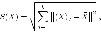
This function calculates the size of the centroid and the baseline size of the certain shape. The centroid size of the shape $S(X)$ is the squared root of the sum of squared Euclidean distances from each landmark to the centroid,

$$S(X)=\sqrt{\sum_{j=1}^{k}\big\Vert(X)_{j}-\bar{X}\big\Vert^{2}} \; ,$$

where $X_{j}$ is the $j$th row of $X(j=1,...,k)$ and $\bar{X}=(\bar{X_{1}},...,\bar{X_{m}})$ is the centroid.

It must be noted that coincident landmarks are not allowed.

The baseline of the shape is the length between landmarks 1 and 2. The landmark coordinates of the shape should be in the frame <coord>. On the output you will get size of the centroid in the field given with the switch -fout and the baseline size in the field given with the switch -fout2. The centroid size could also be used in a normalized form, $S(X)/\sqrt{k}$, and this would be particularly appropriate when comparing shapes with different numbers of landmarks. Thus, when switch -norm is on function will calculate the size of the centroid in a normalized form.

NDA> centroid -d coord -fout size -fout2 base
NDA> ls
sys
macros
coord
size
base

Calculation of Bookstein coordinates of shape

bookstein	Calculate Bookstein coordinates
-d <coord>	shape's coordinates
-dout <book>	bookstein coordinates

This function calculates the bookstein coordinates of the certain shape.

Let $(x_{j},y_{j}), j=1,..,k$ be $k>2$ landmarks in a plane ($m=2$ dimensions). Bookstein suggests removing the similarity transformations by translating, rotating and rescaling such that landmarks 1 and 2 are sent to a fixed position. Thus, bookstein coordinates $(u_{j}^{B},v_{j}^{B})^{T}, j=3,...k$, are the remaining coordinates of an object after translating, rotating and rescaling the baseline to (-0.5,0) and (0.5,0).

In the frame <coord> should be the coordinates of the shape in order (1,2,3,...,k), and coincident landmarks are not allowed. After calculations the new, bookstein coordinates, will be in the frame <book>.

NDA> bookstein -d coord -dout book
NDA> ls
sys
macros
coord
book

Calculation of full Procrustes fit (superimposition) of one shape to another

procrustes	Full Procrustes fit
-d1 <y>	first shape coordinates (centred)
-d2 <w>	second shape coordinates (centred)
-dout <fit>	Procrustes fit (scale, angle and distance)
-dout2 <new>	new coordinates of the second shape

Consider two centred configurations $y=(y_{1},...,y_{k})^{T}$ and $w=(w_{1},...,w_{k})^{T}$. In order to compare the configurations in shape we need to establish a measure of distance between the two shapes. A suitable procedure is to match $w$ to $y$ using the similarity transformations and the differences between the fitted and observed $y$ indicate the magnitude of the difference in shape between $w$ and $y$.

Consider the complex regression equation

$$y=(a+ib)1_{k}+\beta e^{i\theta}w+\epsilon$$

with translation $(a+ib)1_{k}$, scale $\beta$ and rotation $0\leq\theta\leq2\pi$; $\epsilon$ is complex error vector.

This function calculates the full Procrustes fit (superimposition) of one shape ($w$) to another shape ($y$). Which is

$$w^{P}=(\widehat{a}+i\widehat{b})1_{k}+\widehat{\beta}e^{i\widehat{\theta}}w$$

where $(\beta, \theta, a, b)$ are chosen to minimize squared distance

$$D^{2}(y,w)=\Vert y-w\beta e^{i\theta}-(a+ib)1_{k}\Vert^{2}$$

Thus, the coordinates of the shapes $y$ and $w$ have to be centred and in order. Coincident landmarks are not allowed. In the output frame <fit> there will be three fields, scale ($\beta$), angle ($\theta$) and distance (full Procrustes distance). New coordinates of the fitted shape <w> will be stored in the frame <new>.

NDA>procrustes -d1 y -d2 w -dout fit -dout2 new
NDA>ls -fr fit
fit.scale
fit.angle
fit.distance

Centering of landmarks' coordinates of shape

centering	Centering of the coordinates
-d <coord>	shape coordinates
-dout <new>	centred coordinates

This function fulfill centering of the landmarks' coordinates of the shape given in the frame <coord>. Coincident landmarks are not allowed. New coordinates will be stored in the frame <new>.

NDA>centering -d coord -dout new