The basic data management operations are used for managing the Name space and basic data types. These operations can be categorized as follows:
| md | Create a new subdirectory |
| <dirname> | name of subdirectory to be created |
| mkdir | Create a new subdirectory |
| <dirname> | name of subdirectory to be created |
| rd | Remove a subdirectory |
| <dirname> | name of subdirectory to be removed |
| rmdir | Remove a subdirectory |
| <dirname> | name of subdirectory to be removed |
| cd | Change the current directory |
| <dirname> | name of subdirectory to move to |
| pwd | Print current working directory |
This set of commands is meant for managing subdirectories. The directory system has the same principle as file systems. Directories can be created with md (or mkdir) and they can be removed with rd (or rmdir). The NDA kernel keeps track of the current working directory, which can be changed with cd command.
Subdirectories should always be created with md (or mkdir), but items can be referred to by giving the whole (absolute) or relative path of the name entry, for instance, /tmp/first/data or ../first/data (if the current working directory is /tmp/second, for instance). A subdirectory needs to be empty before it can be deleted with rd (or rmdir).
Example: Boston data set contains information about appartments sold in Boston, MA during a certain time period. There are lots of properties, which can be used for truly thorough analyses. If one would want to perform a similar analysis for certain parts of the original data set, it can be easily performed with directories and selrec (see section 4.4.3).
NDA> load boston.dat
...
# Split boston data into two parts
NDA> md part1
NDA> md part2
NDA> selrec -d boston -expr 'boston.rate' < 40; -dout part1/data
NDA> selrec -d boston -expr 'boston.rate' >= 40; -dout part2/data
NDA> cd part1
NDA> runcmd analysis
# Data analysis for low-priced appartments
...
NDA> cd ../part2
# Could perform data analysis for more expensive appartments
...
References to name entries in different directories can be made using absolute or relative paths. This example also shows that only an empty directory can be removed.
...
# Referencing name entries in different directories
NDA> ls ../part1 -fr *
 data
 data.crim
 data.zn
...
NDA> cd ..
NDA> somtr -d part1/prep -sout som2 -l 4
...
NDA> rd part2
 Returned error -134: Try to remove a directory that is not empty
# Error caused by the deletion of a non-empty subdirectory.
# Thus let's remove items under it first
NDA> rm part2/data
NDA> rd part2
| ls | List names in the name space |
| [-d] | limit list to data frames |
| [-c] | limit list to cldata frames |
| [-st] | limit list to structures |
| [-stn <stnum>] | limit list to structures where usage is <stnum> |
| [-fr <frame>] | list the entries in a frame; wildcard * for frame name is available |
| [-sd] | list names in subdirectories |
| [-r] | list recursively all subdirectories of chosen or current directory |
| [-u] | print usage for each listed entry |
| [-t] | print the types of entries |
| [-p] | print the full paths of listed names |
| [-l] | print usage, type and full path for each listed entry |
| [-f] | print only field names with the flag '-fr' |
| [-fout <fld>] | write output into a string field, <fld>, instead of the terminal |
| [<dirname>] | name of the subdirectory to be listed |
This command can be used to list the contents of the name space. The sys structure is part of the name space and always present in the root directory. It cannot even be deleted. Types include st(ructure), dir(ectory), fr(ame), int(eger field), float (field), etc.
Example: The Boston data is loaded and then the contents of the name space (or part of it) is listed in a couple of different ways.
NDA> load boston.dat
NDA> ls
 .
 sys
 boston
NDA> ls -fr boston
 boston.crim
 boston.zn
...
# Listing types and usages with the names (-l does the same)
NDA> ls -t -u -p
 dir  dir  /.
 st   10   /sys
 fr   d    /boston
| rm | Remove entries from the name space |
| <name> | | remove a name entry (any type, but no references to it) |
| -fr <frame> <item> | | remove an item from a frame |
| -ref <item> | | cut all the links to an item and delete it |
| -r <dir> | recursive deleting; wildcard * can also be used |
This command removes name entries: fields, frames, structures and links between the frames and items. The basic command rm removes a name entry, which is not referred to by other frames. Instead of the general usage, you can also remove referred items with the flag -ref when all the links are deleted automatically. Also with the flag -fr an item can be deleted if the reference is the last one. With -r you can recursively delete directories and their contents. The sys structure is part of the name space and cannot be deleted.
Example:
NDA> load boston.dat
...
# Remove the reference to a field from a frame, but do not delete
# the field itself, if it is referred to by other frames
NDA> rm -fr boston boston.crim
...
# Remove a frame and all otherwise unreferenced fields under it
NDA> rm boston
...
# Remove a structure
NDA> rm som1
...
# Clear the name space
NDA> cd /
NDA> rm -r *
| ren | Rename a name entry |
| <oldname> | old name |
| <newname> | new name |
Name entries can be renamed with this command.
Example:
NDA> load boston.dat
NDA> ls
 .
 sys
 boston
NDA> ren boston town
NDA> ls
 .
 sys
 town
| copy | Copy a data frame into a new one |
| <source> | name of source data |
| <target> | name of target data |
| copy | Copy a field instead of a frame |
| -f <srcfld> <trgfld> |
This command copies a source data frame (or field) into a target frame (or field) leaving the original frame intact. In the case of frames, the data fields are also copied instead of just creating new references (see select in section 2.9).
Example:
NDA> load boston.dat
NDA> copy boston data2
NDA> ls -fr data2
 data2.crim
 data2.zn
...
| getdata | Display the contents of a data frame |
| <name> | name of the data frame or field to be listed |
| [-tab] | use tabular format instead of the old one |
| [-fout <file>] | store tabular output into file instead of return buffer |
Without any switches this command returns the contents of a data frame or field in a buffer and displays it. If <name> refers to a data frame, then the result includes name, type and data values of each field in the frame. If <name> refers to a field, then type and data values of the field are listed.
If -tab switch is used, the output of a field just contains the field values. With this switch the output of a frame is given in tabular form, where the width of each column depends on the contents of the data (columns are adjusted to accomodate even the largest values and longest strings). The first row contains the field names and the others field values. The output of a tabular frame can be redirected into a file with switch -fout.
Example: Boston data and field boston.crim can be listed as follows.
NDA> load boston.dat
NDA> getdata boston
crim
2
13.245000
12.002000
0.001000
30.000000
...
zn
2
1.200030
1.430000
...
NDA> getdata boston.crim
2
13.245000
12.002000
0.001000
30.000000
...
| len | Get the number of data items in a name entry |
| -n <name> | any name |
| -fout <trgfld> | field to be created |
| [-dout <trgdata>] | target data frame |
This command reads the length of data in a name entry and stores it in a specified field, which can be put into a data frame with -dout.
Example: The length of boston.crim can be displayed as follows.
NDA> load boston.dat
NDA> len -n boston.crim -fout blen
NDA> getdata blen
1
506
| setdata | Put data values according to indexes into a data field |
| -f <fldname> | field to be modified |
| -vals <index> = <value> ...; | index - value pairs |
| [-len <len>] | length of the field to be created |
| [-t <type>] | type of the field to be created |
This command places specified data values according to indexes into a specified data field. The values are given as index - value pairs. If a field does not exist, then the parameters <len> and <type> must be given. The type is specified with one of the strings int, float or string. Note, that a strong conversion is used. This means that if an integer is given for a string field, the value is handled as a string, and the same holds for all other data types. Vector elements, whose value is not specified, receive a zero or empty value.
Example: In the following examples, the range (min/max) is computed using fldstat (see section 4.7) into frame minmax. The first field contains the minimum and the second field the maximum values for each original field. Therefore, index 0 of frame minmax refers to the first field in the source data (boston.criminality). Thus, the operation setdata forces the minimum value for criminality to 5 and maximum to 50.
NDA> load boston.dat
NDA> fldstat -d boston -dout minmax -min -max
NDA> ls -fr minmax
 minmax.min
 minmax.max
NDA> setdata -f minmax.min -vals 0=5;
NDA> setdata -f minmax.max -vals 0=50;
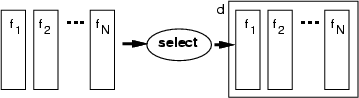
| select | Select fields to a frame |
| <data> | name of the data frame |
| -f <field-list> | fields to be selected |
This operation connects fields into a data frame, which will be created, if it does not exist. The command can also be used to add more fields to an existing frame as the example below shows.
| select | Select all fields from a data frame into a target frame |
| <data> | name of the target data frame |
| -d <src-name> | source data frame |
This operation connects all the fields from a given frame to a target frame.
Example: Names in the name space are listed with ls and then two fields get selected to the new frame data2. Thereafter, an additional field is added to data2.
NDA> load boston.dat
NDA> ls -u -fr
 d    boston
 f    boston.crim
 f    boston.zn
 f    boston.indus
 f    boston.chas
...
NDA> select data2 -f boston.crim boston.zn
# Select more fields
NDA> select data2 -f boston.indus
NDA> ls -fr data2
 data2.crim
 data2.zn
 data2.indus
# Select all fields from a given data
NDA> select data3 -d boston
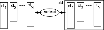
| select | Select classes to a classified data frame |
| <cldata> | classified data frame |
| -cl <class-list> | classes to be selected |
This operation connects classes to a classified data frame. If a frame does not exist, it will be created. The command can also be used to add classes to an existing classified data frame.
| select | Select classes from a classified data |
| <cldata> | classified data frame |
| -c <cldata-src> | name of the classified data |
This operation collects all the classes of a specified classified data frame to a target classified data.
Example (ex2.1): The command select has been used to connect two classes class1 and class3 to a new classified data cldata2. (For creating classes see section 2.13.) You can first run the example `ex2.1' and then apply the following commands:
...
# Create data classes
NDA> addcld...
...
NDA> ls -u -fr
...
 c    cldata1
 cl   cldata1.class1
 cl   cldata1.class2
 cl   cldata1.class3
NDA> select cldata2 -cl cldata1.class1 cldata1.class3
# Add more classes
NDA> select cldata2 -cl cldata1.class2
NDA> select cldata3 -c cldata1
| select | Select classes to a classified data frame |
| <frame> | name of the frame (any type) |
| -n <item-name> | item(s) to be selected |
This operation connects any possible item(s) to a frame and no type checking is done. Thus, the operation can also be used with data and classified data frames. It is also necessary to use this option, if fields of variable length are collected into a data frame.
Example: Membership functions of fuzzy sets are described as data fields of variable length. The following example demonstrates how some part of defined fuzzy sets can be selected to compute fuzzy values for the data values later. (For creating fuzzy sets, see section 4.9.1 and related topics.)
...
# Create a fuzzy structure and sets
NDA> mkfz fz1...
...
NDA> ls -fr fz1
 fz1.sets
 fz1.sets.small
 fz1.sets.medium
 fz1.sets.large
 fz1.ranges
...
NDA> select fz2.sets -n fz1.sets.small fz1.sets.large
...
NDA> calcfz fz2 -f boston.dis -dout dis_fuzzy
| attchdat | Attach a data frame to the end of another frame |
| -d <data> | name of the source data (data to be attached) |
| -dout <target-data> | name of the target data |
This command attaches another data frame to target data. New data records are added after existing data records in the target data, and the operation assumes that there are existing data records available in the target data. Naturally, the types and lengths of the data frames have to match, which is also checked.
Example: The example duplicates the Boston housing data.
NDA> load boston.dat
NDA> copy boston data2
NDA> attchdat -dout data2 -d boston
# Now data2 contains duplicated data records
| addcld | Create an empty classified data |
| -c <cldata> | name of the classified data |
| addcl | Add a new class to classified data |
| -c <cldata> | classified data |
| -cl <class> | name of the new class |
| updcl | Update a class by an identifier |
| -cl <class> | name of the class |
| -id <id> | an identifier |
| cpcld | Copy a classified data frame |
| -c <cldata> | source frame |
| -cout <cldataout> | target frame |
| cpcl | Copy a single class |
| -cl <class> | source class |
| -cout <cldata> | target classified data |
| -clout <classtrg> | target class |
| shftcld | Shift indexes in a classified data |
| -c <cldata> | source classified data |
| [-id <shift-id>] | the number to be added to indexes |
| [-cout <cldata>] | target classified data (source is used, if this is omitted) |
These commands are meant for handling classified data frames. addcld creates an empty classified data frame. addcl creates a new empty class to a classified data. updcl updates a class with an identifier. The identifier is created to the class, if it does not exist, otherwise the identifier is removed from the class. shftcld adds a constant index to all the indexes in a classified data (or 0 if -id is omitted).
Example (ex2.2): A typical use for these commands is grouping of SOM neurons. The whole grouping is placed into a classified data frame, in which each class corresponds to one group of neurons.
NDA> somtr...
...
NDA> addcld -c groups
NDA> addcl -c groups -cl goodAp
NDA> updcl -cl groups.goodAp -id 14
NDA> updcl -cl groups.goodAp -id 16
NDA> addcl -c groups -cl badAp
NDA> updcl -cl groups.badAp -id 17
# Remove 17 from badAp
NDA> updcl -cl groups.badAp -id 17
Example: Normally, the grouping is not performed manually but with the graphical user interface (GUI). The following command sequence describes, what happens behind the GUI.
The identifiers of the neurons are got from a graphical image by the commands fndpnt and fndreg (see section 8.14.2). This can also be invoked by runevent (see section 8.14.3). Typically the coordinates for these commands are got from a mouse event. First you should run the example `ex7.4' and then apply the following commands:
...
# When a window is opened:
# Create a grouping and a group (if they do not exist)
NDA> addcld -c som1Grp
NDA> addcl -c som1Grp -cl goodAp
...
# A mouse click event causes the following commands to be run:
# For updating a single neuron to current group
NDA> fndpnt grp1 0.3 0.4
# -> neuron id = 8
NDA> updcl -cl som1Grp.goodAp -id 8
...
# A mouse choose_region event causes the following commands:
# For updating a region of neurons to current group
NDA> fndreg grp1 0.1 0.1 0.5 0.1 0.5 0.5 0.1 0.5
# -> neuron ids = 8, 6, 5, 7
NDA> updcl -cl som1Grp.goodAp -id 6
NDA> updcl -cl som1Grp.goodAp -id 5
NDA> updcl -cl som1Grp.goodAp -id 7
| serie | Create a series of numbers |
| {-d <data> | existing data, |
| | -len <length>} | or length of the field, alternatively |
| -fout <field-name> | field to be generated |
| [-start <start-value>] | minimum value for series (or 0) |
| [-step <step-value>] | step between the values (or 1) |
This command creates a new data field by generating numeric values. The values are created by starting from the <start-value>, and by increasing the generated value by <step-value> each time. The <step-value> can be zero or negative, too. Length of the resulted field can be given through the reference data or as a parameter.
Example: The following example demonstrates how identifiers can be generated for data records.
NDA> load boston.dat
NDA> serie -d boston -fout boston.id -start 0 -step 1
NDA> getdata boston.id
1                           # Type = 1 (integer)
0                           # The created series
1
2
3
...
| flds2str | Pack fields to one string field |
| -d <data> | existing data frame |
| -fout <field-name> | field to be generated |
| [-sep <separator>] | separator to be used between fields |
This command packs all data fields of <data> as a string into one new data field, which is created using <field-name>. The values are packed in the same order in which they lie inside the data frame and <separator> is used between the values.
Example (ex2.4): The following example demonstrates how two fields of the Boston data can be packed into one field that is used to label the neurons of a SOM. Neurons are labelled with reclab (see section 8.4.10).
NDA> load boston.dat
...
# Here the Boston data is analyzed using TS-SOM
# and the SOM is visualized in window "win1"
NDA> select labflds -f boston.chas boston.crim
NDA> flds2str -d labflds -dout labs -sep _
NDA> reclab win1 -f labs -max 5
| sec2time | Convert seconds to time format |
| -f <sec-field> | field containing seconds |
| -fout <time-field> | field to be created |
| [-sep <separator>] | separator |
| time2sec | Convert time format to seconds |
| -f <time-field> | field including seconds |
| -fout <sec-field> | field to be created |
| [-sep <separator>] | separator |
The command converts seconds to a time format. Seconds are represented as integers, and the time format as a string. The separator in the time format is optional with the default value `:'. Thus, the default time format is hh:mm:ss.
Example: The example shows, how conversions between seconds and the time format can be performed.
...
NDA> getdata time1
3
12:34:56
NDA> time2sec -f time1 -fout secs
NDA> getdata secs
1
45296
NDA> sec2time -f secs -fout time2 -sep .
NDA> getdata time2
3
12.34.56
Matrix is a data structure initially designed for multi-dimensional calculations with the Fourier transform method. However, the matrix design also allows normal vectors to be stored in matrix form.
To perform any of matrix operations with some data stored in a data frame, it first needs to be converted into matrix form by applying a special command (data2mat, d2m or f2m). These commands will create a two (or one) dimensional matrix. All the other commands described below can be applied only to two-dimensional matrices.
REMARKS! You cannot save a matrix directly. Thus, it first needs to be converted into a data frame (mat2data or m2d) and then saved using the command save (see section 9.2).
There are two basic user commands for matrices in addition to the conversion routines:
| matrix | Create a small one or two dimensional matrix |
| <name> | name of the input data |
| <[a, b;c, d]> | input values |
| Print the contents of a matrix | |
| <matr> | matrix or field to be printed |
| [-matr] | choose matrix mode |
| [-f] | choose field mode |
The command matrix is used to create a small one or two dimensional matrix manually. The matrix created with this command contains only float values.
Matrix contents can be viewed by using the command print. This command can also be used to print integer and float fields. The values are printed using the following order: 1. [0]...[0][0][0-n], 2. [0]...[0][1][0-n], ...
| d2m | Convert a data frame into the framed matrix form |
| -d <data> | data frame to convert |
| -mout <matr> | name of the destination framed matrix |
| -dim <n> <d1>...<dn> | n is the number of dimensions and d? is the length of each dimension |
| f2m | Convert a data field to the matrix form |
| -f <field> | data field to convert |
| -mout <matr> | name of the destination framed matrix (a matrix containing only one line) |
| m2d | Convert a matrix to a data frame |
| -m <matr> | framed matrix to convert |
| -dout <data> | destination data frame |
| shape | Change the shape of a matrix |
| -m <matr> | input framed matrix |
| -mout <matr> | name of the destination framed matrix |
| -dim <n> <d1>...<dn> | n is the number of dimensions and d? is the length of each dimension |
These commands are used to manipulate the data structures in the NDA, especially matrices that have been put into a frame. The data frame for d2m can contain several fields, each of these fields is converted into a matrix structure. The command f2m converts only one field into a matrix. The default form of one line containing all field items is used. The command m2d converts a matrix into a normal data frame, which can be saved or used with other NDA commands. The command shape is used for changing the dimensions of matrices. The matrices are actually data frames with fields defined as matrix structures.
Example (ex2.3): This example shows how these commands can be used for changing the data format inside the NDA.
NDA> load sin.dat
# Change data fields into 2x10 matrices (mat.x and mat.y)
NDA> d2m -d sin -mout mat -dim 2 2 10
# Change field sin.x into a 1x20 matrix.
NDA> f2m -f sin.x -mout matx
# Create a new matrix from "mat" with different shape
NDA> shape -m matx -mout matr -dim 2 4 5
# Create a new data frame from the matrix
NDA> m2d -m matr -dout data
# Save the new data frame
NDA> save data
| data2mat | Convert a data frame into a matrix |
| -d <data> | name of the data frame |
| -mout <matr> | name for the destination matrix |
The command data2mat converts a data frame into a two-dimensional matrix. The dimension of the output matrix is the same as the dimension of the input data frame. The number of rows of the matrix corresponds to the number of data records in the frame, and the number of columns corresponds to the number of fields.
| mat2data | Convert a matrix into a data frame |
| -m <matr> | name of the matrix given |
| -dout <data> | name for the destination data frame |
The command mat2data performs the reverse operation compared to data2mat, it converts a matrix into a data frame. It should be mentioned that matrix conversion operations do not preserve the names of the fields of the original data frame. Instead, the fields are named field_<n>. Integer fields are also converted into floats.
NDA> load data.dat
-field <f1> -len(2)
-field <f2> -len(2)
-field <f3> -len(2)
-field <f4> -len(2)
# Change data fields into matrix
NDA> data2mat -d data -mout mat
NDA> mat2data -m mat -dout new_data
NDA>ls -fr new_data
new_data.field_0
new_data.field_1
new_data.field_2
new_data.field_3
NDA> save new_data
| svd | Performs Singular Value Decomposition for the given matrix |
| -m <matr> | name of the matrix |
| [-u <u_mat>] | name of the column-ortogonal left matrix (default name U_matrix) |
| [-w <w_mat>] | name of the diagonal matrix with singular values (default name W_matrix) |
| [-v <v_mat>] | name of the ortogonal right matrix (default name V_matrix) |
The command svd performs a singular value decomposition of the given matrix. The formal definition of SVD is as follows: Given an ![]() real matrix
real matrix ![]() , where the
, where the ![]() is the number of rows and the
is the number of rows and the ![]() the number of columns, we can express it as:
the number of columns, we can express it as:
![]() , where
, where ![]() is a column-orthonormal
is a column-orthonormal ![]() matrix or left matrix, where
matrix or left matrix, where ![]() is the rank of the matrix
is the rank of the matrix ![]() ,
, ![]() is a diagonal
is a diagonal ![]() matrix, and
matrix, and ![]() is a column-orthonormal
is a column-orthonormal ![]() matrix or right matrix. The matrix
matrix or right matrix. The matrix ![]() is called column-orthonormal if its columns are mutually orthonormal unit vectors. Equivalently:
is called column-orthonormal if its columns are mutually orthonormal unit vectors. Equivalently:
![]() , where
, where ![]() is the identity matrix. The rank of the matrix is the highest number of linearly independent rows (or columns). For the simplicity for svd the value of
is the identity matrix. The rank of the matrix is the highest number of linearly independent rows (or columns). For the simplicity for svd the value of ![]() is equal to the number of columns in matrix
is equal to the number of columns in matrix ![]() . Thus, if the rank of the matrix is smaller than the number of columns, some columns and rows are zero vectors. In other words, dimensions of the matrix are for
. Thus, if the rank of the matrix is smaller than the number of columns, some columns and rows are zero vectors. In other words, dimensions of the matrix are for ![]() :
: ![]() , for
, for ![]() :
: ![]() , and for
, and for ![]() :
: ![]() .
.
By default the left matrix, the right matrix, and the diagonal matrix containing the singular values will get names U_matrix, V_matrix and W_matrix correspondingly.
| pinv | Calculate the pseudo-inverse matrix for the given matrix |
| -m <matr> | name of the given matrix |
| -mout <pseudo> | name for the pseudo-inverse matrix |
The command pinv calculates a pseudo-inverse matrix of the given matrix. For the given ![]() matrix
matrix ![]() , the pseudo-inverse matrix is defined as:
, the pseudo-inverse matrix is defined as:
![]() . Also note that:
. Also note that:
![]() , but
, but
![]() in general. In the square matrix case this command gives us an inverse matrix of the given matrix.
in general. In the square matrix case this command gives us an inverse matrix of the given matrix.
| lu | Performs LU-decomposition for the given matrix |
| -m <matr> | name of the square matrix |
| [-l <l_mat>] | name for the lower-triangular matrix (default name lower_triang) |
| [-u <u_mat>] | name for the upper-triangular matrix (default name upper_triang) |
| [-fout <f_det>] | name for the determinant of the given matrix (default name determinant) |
The command lu performs an LU decomposition of the square matrix and its definition is: ![]() , where
, where ![]() is the given
is the given ![]() matrix,
matrix, ![]() is the lower-triangular matrix, and
is the lower-triangular matrix, and ![]() is the upper-triangular matrix. The determinant of the matrix is also calculated. By default, the name of the lower-triangular matrix will be lower_triang, and the name of the upper-triangular matrix will be upper_triang in the NDA namespace. The value of the determinant, by default, will be stored in the field named determinant.
is the upper-triangular matrix. The determinant of the matrix is also calculated. By default, the name of the lower-triangular matrix will be lower_triang, and the name of the upper-triangular matrix will be upper_triang in the NDA namespace. The value of the determinant, by default, will be stored in the field named determinant.
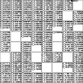
Example: Here is a simple example for svd, pinv, and lu.
NDA> load data.dat
# Change data fields into matrix
NDA> data2mat -d data -mout mat
# Calculate SVD, pseudo-inverse and LU decomposition
NDA> svd -m mat
NDA> pinv -m mat -mout pseudo
NDA> lu -m mat
NDA> ls
  sys
  macros
  data
  mat
  U_matrix
  W_matrix
  V_matrix
  pseudo
  lower_triang
  upper_triang
  determinant
| m+m | Calculate the sum of two matrices |
| -m1 <matr1> | name of the first matrix |
| -m2 <matr2> | name of the second matrix |
| -mout <result> | name for the result matrix |
This command calculates the sum of two given matrices. Note that the dimensions of those matrices must be the same.
| m-m | Subtract one matrix from another |
| -m1 <matr> | name of the first matrix |
| -m2 <matr> | name of the second matrix |
| -mout <result> | name for the result matrix |
This command subtracts matrix <matr2> from matrix <matr1>. Note that the dimensions of those matrices must be the same.
| mxm | Multiply two given matrices |
| -m1 <matr1> | name of the first matrix |
| -m2 <matr2> | name of the second matrix |
| -mout <result> | name for the result matrix |
This command multiplies two given matrices. The number of columns in the first matrix <matr1> must be equal to the number of rows in the second matrix <matr2>.
| mxnum | Multiply a matrix by a number |
| -m <matr> | name of the matrix |
| -num <number> | the number |
| -mout <result> | name for the result matrix |
This command multiplies each item of the given matrix by a number.
| trans | Transpose the given matrix |
| -m <matr> | name of the given matrix |
| -mout <transpose> | name for the transpose of the matrix |
This command calculates the transpose of the given matrix.
| inverse | Calculate the inverse of the given matrix |
| -m <matr> | name of the given matrix |
| -mout <transpose> | name for the inverse of the matrix |
| [-iter <num_iter>] | maximum number of iterations (default 100) |
| [-eps <epsilon>] | minimum change (default 0.000001) |
This command calculates the inverse of the given matrix. The method is iterative and the maximum number of iterations can be specified. The iteration is also terminated if the resulting matrix does not change more than <epsilon> between iterations.
| chol | Calculate the Cholesky decomposition of the given matrix |
| -m <matr> | name of the given matrix |
| -mout <transpose> | name for the resulting matrix |
This command calculates the Cholesky decomposition of the given matrix.