The basic data computing includes operations for simple calculation. There are two main groups of such operations. The first group is meant for basic computing of data fields through the so-called field evaluator. The second group includes operations for basic statistics of either fields or classes.
Preprocessing includes operations for data equalization, data normalization, whitening, data record equalization and treatment of missing data.
| prepro | Macro command for preprocessing |
| -d <data> | the name of the data |
| -dout <dataout> | result data |
| [-e] | min/max based equalization of fields |
| [-edev] | variance-based equalization of fields |
| [-n] | normalization of data records |
| [-d2 <equdata>] | statistical values to be used for equalization |
| [-md <value>] | missing value to be skipped |
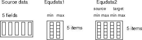
Purpose of preprocessing is to eliminate such statistical properties of data, which are caused by data coding. These properties have often an undesired effect to dimensionality reduction algorithms. prepro is a macro operation including several suboperations to preprocess the data. It takes a data frame as input and produces a new data frame as output. The suboperations can be selected according to the flags as follows:
If <equdata> is not given then ![]() and
and ![]() are defined according to the range of the source data (from the field
are defined according to the range of the source data (from the field ![]() ), and the target range
), and the target range
![]() is set to [0,1]. In this case, the scaling formula can be simplified to the form:
is set to [0,1]. In this case, the scaling formula can be simplified to the form:
If <equdata> contains only two fields, then these fields are used as a source range (equdata 1 in the figure below). And the values ![]() (1. field) and
(1. field) and ![]() (2. field) are read from <equdata> (the index of the field in source data corresponds to the index of data record in <equdata>). The fields in <equdata> should have a length matching the number of fields in the data to be processed. If <equdata> contains four fields (see equdata 2 in the figure below), then all the scaling information is read from this data. In this case, the order of fields in <equdata> is
(2. field) are read from <equdata> (the index of the field in source data corresponds to the index of data record in <equdata>). The fields in <equdata> should have a length matching the number of fields in the data to be processed. If <equdata> contains four fields (see equdata 2 in the figure below), then all the scaling information is read from this data. In this case, the order of fields in <equdata> is
![]() .
.
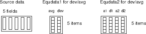
Similarly to the ![]() -based equalization, the scales can be computed directly from the source data or read from a frame. In the first case, for each field, the average value and standard deviation are computed before the field is scaled. In the second case,
-based equalization, the scales can be computed directly from the source data or read from a frame. In the first case, for each field, the average value and standard deviation are computed before the field is scaled. In the second case, ![]() and
and ![]() can be given in <equdata> (see the figure below). The first field in this data should contain
can be given in <equdata> (see the figure below). The first field in this data should contain ![]() and the second field
and the second field ![]() . Also, it is possible to specify the target average and deviation through <equdata> (see equdata 2 in the figure below). In that case, data fields are scaled as follows:
. Also, it is possible to specify the target average and deviation through <equdata> (see equdata 2 in the figure below). In that case, data fields are scaled as follows:
where ![]() and
and ![]() contain the statistics of source data, and
contain the statistics of source data, and ![]() and
and ![]() specify the target ranges of data fields.
specify the target ranges of data fields.
Example (ex4.1): Typically, prepro is used with SOM operations somtr and somcl. This example demonstrates how data is preprocessed and the SOM is trained with the preprocessed data.
...
NDA> prepro -d boston -dout predata -e -n
NDA> somtr -d predata -sout som1 -l 4
...
Example: If a SOM is used as a classifier, it is important that new, unseen data records are preprocessed the same way as training data. Thus, it is necessary to save the statistics of original data so that the same equalization can be performed later. The following commands demonstrate this for the ![]() -based equalization, but the same procedure can also be applied to the deviation-based equalization. In that case, the averages and deviations should be computed instead of the minimum and maximum values.
-based equalization, but the same procedure can also be applied to the deviation-based equalization. In that case, the averages and deviations should be computed instead of the minimum and maximum values.
# Load the Boston data and take a sample for training a SOM
NDA> load boston.dat
NDA> selrec -d boston -dout sample1 -expr 'boston.rm' > 5;
# Compute min/max info, save it and use it in preprocess
NDA> fldstat -d sample1 -dout mminfo -min -max
NDA> save mminfo -o mminfo.dat
NDA> prepro -d sample1 -dout predata -d2 mminfo -e -n
NDA> somtr -d predata -sout som1 -l 4
...
NDA> save som1 -o som1.som
...
# Shutdown the NDA and start it again for matching
# the whole data to our sample
NDA> load boston.dat
NDA> load mminfo.dat
NDA> load som1.som
# Preprocess data and classify it with the SOM
NDA> prepro -d boston -dout predata -d2 mminfo -e -n
NDA> somcl -d predata -s som1 -cout cld
NDA> clstat -d boston -dout sta -c cld -hits -avg -min -max
# Continue visualization for exploring the mapped data
...
| whitening | Whitening transformation |
| -d <data> | data frame to be preprocessed |
| -dout <dataout> | name of the preprocessed data frame |
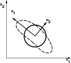
The whitening transformation is a linear preprocessing method which allows correlation among variables. The transformation is performed using eigenvectors from covariance matrix in a way that is illustrated roughly in the figure below. Data frame to be processed may only contain floating point vectors. This transformation is useful, if source data contains fields, which differ a lot in magnitude.
Example (ex4.12): Load some arbitrary data and perform the whitening transformation.
# Load some data in
NDA> load sin.dat
# Perform the whitening transformation
NDA> whitening -d sin -dout whitesin
| equrec | Equalize values of data records |
| -d <data> | data frame to be preprocessed |
| -dout <dataout> | name of the preprocessed data frame |
| [-min <minval>] | minimum value for target range (default 0) |
| [-max <maxval>] | maximum value for target range (default 1) |
| [-global] | should variance and average be used or just minimum and maximum |
This operation equalizes values of each data record into range [minval,maxval]. In the normal case, it first locates the minimum and the maximum values from each data record and then all the values are scaled linearly from ![]() to the specified (or unit) range. If -global is specified, the operation first calculates the variance of data record average values and then updates the values with the following equation:
to the specified (or unit) range. If -global is specified, the operation first calculates the variance of data record average values and then updates the values with the following equation:
For an example, see concseq (section 3.18).
| msd | Replace missing data |
| -d <datain> | source data frame |
| -dout <dataout> | target data frame |
| [-ddist <distdata>] | distance data (if different from source) |
| [-md <value>] | the missing value (default -9999.0) |
| [-num <maxmf>] | maximum number of missing fields / data record |
| [-ver] | verbose reporting of replacements and discarded records |
| [-stat] | report number of original, completed and discarded data records, minimum and maximum located distance etc. |
| msdbycen | Replace missing data with prototypes |
| -d <data> | source data frame |
| -d2 <proto-data> | prototype data |
| -c <cldata> | connections from prototypes |
| -dout <dataout> | the name of the replaced data frame |
| -md <value> | the missing value |
| [-ver] | verbose |
Operation msd replaces all missing values from the source data by using the field values found from the nearest data record. The nearest data record is determined by using the normalized distance that is computed according to the following formula:
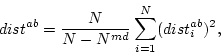
where ![]() is the number of such components, from which value is missing in
is the number of such components, from which value is missing in ![]() or in
or in ![]() , and
, and ![]() is the total number of data fields. The computation of the distance recognizes the number of missing values and scales the distances in a way that the pairs of the data records containing lots of missing values get larger distances. The located nearest data record may not contain missing values in the same fields as the one being completed.
is the total number of data fields. The computation of the distance recognizes the number of missing values and scales the distances in a way that the pairs of the data records containing lots of missing values get larger distances. The located nearest data record may not contain missing values in the same fields as the one being completed.
If the maximum number of missing fields is specified, all data records having more missing fields are discarded from the output data frame. Also records that cannot be completed are discarded. The missing data value can be specified and also a separate frame to be used as a distance data. Statistics and even verbose processing of data records containing missing fields can be requested.
The operation msdbycen replaces missing values with the values of prototypes given in a separate data frame. The classified data frame should indicate, which data records are connected to which prototypes. See also somcl (section 5.1.2) about the missing data flag.
Example: Remove missing fields (marked with -9) from source data, but do not allow more than 4 missing fields / record.
# Load data containing missing fields
NDA> load kv.dat -n km
# Perform missing data removal
NDA> msd -d km -dout kv -md -9 -num 4 -stat
 distances: min   16.6/  515.4, max   92.2/  847.7
 - data rec: src 1120, corrected 130, discarded 28 => trg 1092
| gen | Generate random data from uniform or normal distribution |
| -U <bgn> <end> | -N <exp> <var> | distribution; either uniform distribution from <bgn> to <end> or normal distribution with expectation value <exp> and variance <var> |
| -dout <dataout> | output data frame |
| -s <samples> | number of samples |
| [-dim <dim>] | dimension (default is 1) |
This command generates samples from the specified distribution and saves them to the namespace. Data frame <dataout> contains <dim> fields, i.e. one field for each dimension. Fields are named F0, F1, etc.
Example: Generate 200 random numbers between 3.4 and 5.7,
and 400 samples from a two-dimensional normal distribution.
NDA> gen -U 3.4 5.7 -dout rands -s 200
NDA> gen -N 0 1 -dout gauss -s 400 -dim 2
This special command can be used to create the full or reduced ortogonal DoE (design of experiment) plan for the ![]() factors, each at two levels.
factors, each at two levels.
| plan | Composing ortogonal DoE plan |
| -fac <number> | the number of factors |
| -dout <ortoplan> | name for the output data frame where the plan will be stored |
| [-full] | compose full factorial plan instead of reduced |
If ![]() factors vary at two levels, each complete replicate of the full factorial design has
factors vary at two levels, each complete replicate of the full factorial design has ![]() runs, and the arrangement is called a
runs, and the arrangement is called a ![]() factorial design. The full factorial design is a matrix that contains
factorial design. The full factorial design is a matrix that contains ![]() columns. The levels of factors are coded as -1 and 1, where -1 means that the factor is adjusted to the lowest level and 1 means adjustment to the highest level of the factor.
columns. The levels of factors are coded as -1 and 1, where -1 means that the factor is adjusted to the lowest level and 1 means adjustment to the highest level of the factor.
Example: Here is an example script that creates a full factorial plan for 3 factors.
NDA> plan -fac 3 -dout table -full
 1       1       1
-1       1       1
 1      -1       1
-1      -1       1
 1       1      -1
-1       1      -1
 1      -1      -1
-1      -1      -1
Sometimes it is possibile to reduce the number of runs significantly in the design without any loss of information. For example, if the nature of the phenomenon is linear, or we assume it to be linear. Such a design is called a fractional factorial design of experiments. If the switch -full is not given, function plan creates an orthogonal plan in the folowing manner.
For the given ![]() number of factors the function plan calculates the minimum number of factors,
number of factors the function plan calculates the minimum number of factors, ![]() , for which it creates a full factorial plan. This full factorial plan is used for the creating of the fractional factorial plan for all
, for which it creates a full factorial plan. This full factorial plan is used for the creating of the fractional factorial plan for all ![]() factors. The columns for the additional factors are calculated as a product of some of the columns from the full factorial plan.
factors. The columns for the additional factors are calculated as a product of some of the columns from the full factorial plan.
For example, if the different factors in the plan are marked with numbers (1,2,3,...), the orthogonal plan for the nine factors is as follows:
| 1 | 2 | 3 | 4 | 5=1x2 | 6=1x3 | 7=1x4 | 8=2x3 | 9=2x4 |
NDA> plan -fac 9 -dout table
 1      1      1      1      1      1      1      1      1
-1      1      1      1     -1     -1     -1      1      1
 1     -1      1      1     -1      1      1     -1     -1
-1     -1      1      1      1     -1     -1     -1     -1
 1      1     -1      1      1     -1      1     -1      1
-1      1     -1      1     -1      1     -1     -1      1
 1     -1     -1      1     -1     -1      1      1     -1
-1     -1     -1      1      1      1     -1      1     -1
 1      1      1     -1      1      1     -1      1     -1
-1      1      1     -1     -1     -1      1      1     -1
 1     -1      1     -1     -1      1     -1     -1      1
-1     -1      1     -1      1     -1      1     -1      1
 1      1     -1     -1      1     -1     -1     -1     -1
-1      1     -1     -1     -1      1      1     -1     -1
 1     -1     -1     -1     -1     -1     -1      1      1
-1     -1     -1     -1      1      1      1      1      1
The NDA kernel has a simple parser, which can be used to evaluate expressions. The parser provides three services: parsing given expressions, checking data types and evaluating parsed expressions.
The parser uses a syntax including the following operators and operands:
| Operands | |
| numerical | normal integer or floating point numbers |
| strings | inside double quotes, for instance, "string" |
| boolean | reserved words: TRUE/FALSE (1 / 0) |
| fields | inside single quotes, for instance, 'stats.hits' |
| Special characters | |
| () | the order of evaluation can be changed using parentheses. They may be nested |
| ; | an expression is always terminated with a semicolon (semicolons within double quotes, i.e. strings, are ignored) |
| Operators | |
| + | sum two numeric operands or, if operands are strings, concatenate them |
| subtract the second operand from the first one | |
| multiply two operands | |
| / | divide the first operand by the second one (integer division, if both operands are integer) |
| % | remainder of the integer division (first by second; both operands have to be integer) |
| raise the first operand a to the power of second operand b, i.e. |
|
| =, >, >=, <, <=, != | compare two operands ( |
| AND | take logical and of two operands ( |
| OR | take logical or of two operands ( |
| NOT | take logical not of a boolean value ( |
| ? : | <bool> ? <expr1> : <expr2> evaluates the boolean expression <bool> and if it is TRUE, chooses the result of <expr1>, and if it is FALSE, chooses the the result of <expr2> |
| Data type conversions | |
| FLOAT | convert the following operand to a float value (strings might result in 0.0, booleans 1.0/0.0) |
| INT | convert the following operand to an integer value (strings might result in 0, booleans 1/0) |
| STRING | corvert the following operand to a string (booleans will result in TRUE/FALSE) |
| Arithmetic functions | |
| RAND | return a pseudo-random floating point number between 0.0 and operand |
| IRAND | return an integer pseudo-random number between 0 and operand - 1 |
| ABS | return the absolute value of operand |
| SQRT | calculate
|
| EXP | calculate |
| LN | calculate the natural logarithm of a positive operand |
| LOG | calculate the 10-based logarithm of a positive operand |
| SIN | calculate the sine of the operand (specified in radians) |
| COS | calculate the cosine of the operand (specified in radians) |
| TAN | calculate the tangent of the operand (specified in radians) |
| ARCSIN | evaluate the angle, whose sine is operand (operand must be between -1.0 and 1.0) |
| ARCCOS | evaluate the angle, whose cosine is operand (operand must be between -1.0 and 1.0) |
| ARCTAN | evaluate the angle, whose tangent is operand |
| Name space functions | |
| LEN | evaluate the length of an item in the name space (operand is specified as a string) |
| USAGE | evaluate the usage of an item in the name space (operand is specified as a string) |
| TYPE | evaluate the data type of an item in the name space (operand is specified as a string) |
| Index functions | |
| IMIN | returns the index of the minimum value in a vector (operand must be a numerical vector) |
| IMAX | returns the index of the maximum value in a vector (operand must be a numerical vector) |
| String functions | |
| BEGINS | <str1> BEGINS <str2> checks if <str1> begins with <str2> and returns a boolean result |
| CONTAINS | <str1> CONTAINS <str2> checks if <str1> contains the substring <str2> and returns a boolean result |
| ASCII | returns the ASCII code of the first character of the string given as parameter |
| CHR | returns a string containing one ASCII character (number given as parameter) |
| FORMAT | "<fmt>" FORMAT <value> returns a string containing <value> in specified sprintf() format (<fmt> must be reasonable for the operand and may contain other text, too) |
| BASENAME | extract the actual name from a filename specification, which probably contains directories and extensions (operand must be a string) |
| DIRNAME | extract the directory name from a filename specification, which also contains a name and possibly extensions (operand must be a string) |
| EXTENSION | extract the extension from a filename specification, which contains directories and the name of the file (operand must be a string) |
| SAFENAME | returns a safe filename, where :, / and |
| STRLEN | returns the length of the string given as parameter |
| INDEX | <str1> INDEX <str2> returns the (first) starting index of <str2> in <str1> |
| RINDEX | returns the last(!) starting index of <str2> in <str1> |
| SUBSTR | <str> SUBSTR <a> : <b> returns the substring of length <b> which starts at character position <a> |
| REPLACE | <str> REPLACE <str1> : <str2> replaces all occurences of <str1> by <str2> from the original string <str> |
The string indices are zero based as in the C language.
Type checking is performed after an expression has been parsed to an abstract syntax tree. In addition, the lengths of data fields are checked. When data fields are referred to in an expression, they must be of equal length or the length must be 1, to make the evaluation possible. Namely, the expression is evaluated record by record (index by index), but data fields having a length of 1 are interpreted as scalar variables. Numerical constants can also be used to represent scalar values.
The evaluation result of the expression depends on the operation, which invokes the parser. If the parser is used to compute a new field (command expr), then the returned value of the evaluation can be of any type. Instead, when the parser is used to evaluate the truth-value of some expression, the parsing should produce boolean values. Then, the highest-level operator of the parsing tree should be a comparison or a logical operator.
Example (ex4.2): The following commands use the expression evaluator (see sections 4.4.2, 4.4.3, 4.4.4 and 8.3.6).
...
# Compute new fields
NDA> expr -dout boston -fout znPrice
     -expr 'boston.zn'/'boston.rate';
...
# Select indexes to a new class according to a given rule
NDA> selcl -cout c1/cld -clout bigZn
     -expr ('boston.zn'>3.0) AND ('boston.rate'<25);
...
# Select a new data frame (containing values under the average)
# In this case 'rate.avg' is a used as a scalar variable
NDA> select avgfld -f boston.rate
NDA> fldstat -d avgfld -dout rate -avg
NDA> selrec -d boston -dout data
     -expr ('boston.rate' < 'rate.avg');
...
# Set neurons to be visible according to a given rule
NDA> nvsbl grp1 -expr 'sta.hits'> 0;
| expr | Field calculator |
| -fout <field> | field for storing the result |
| -expr <expr>; | expression to be evaluated |
| [-dout <dataout>] | output data frame for field |
| [-v] | verbose evaluation |
This command works as a data record calculator. A given expression is evaluated in a loop for each data record. The result values are stored in a new field (inside a data frame, if it has been specified). More information about expressions can be found in section 4.4.1.
Example (ex4.3): This example shows some basic operations for fields and an error message.
NDA> load boston.dat
NDA> expr -dout boston -fout znprice
      -expr 'boston.rate' / ('boston.zn'+0.0001);
NDA> expr -dout boston -fout lowCrim -expr 'boston.crim' < 3;
# Cannot divide by string
NDA> expr -dout boston -fout someVar -expr 'boston.dis' / "xxx";
 Returned error -409: Operand type mismatch for operator
| selrec | Select records according to a boolean expression |
| -d <data> | source data frame |
| -dout <dataout> | output data |
| -expr <expr>; | expression to be evaluated |
| [-v] | verbose evaluation |
This command selects those data records into <dataout>, which produce a TRUE value, when the specified boolean expression is evaluated. Note, that the resulting data has the same fields as the source data. The number of data records might be smaller (or even zero), though. The expression must give a boolean value as a result. More information about expressions can be found in section 4.4.1.
Example (ex4.4): This example selects data records, which represent expensive apartments.
NDA> load boston.dat
NDA> selrec -d boston -expr 'boston.rate' > 30; -dout data
# Continue analysis for them
NDA> prepro -d data -dout predata -e -n
NDA> somtr -d predata -sout som1 -l 4
...
| selcl | Select records according to a boolean expression |
| -cout <cldata> | target classified data |
| -clout <class> | class to be created |
| -expr <expr>; | expression to be evaluated |
| [-v] | verbose evaluation |
This command selects the indexes of data records into a new class. It evaluates a given boolean expression for each record, and those records returning the value TRUE are collected to the class. Therefore, the expression must return boolean values. More information about expressions can be found in section 4.4.1.
Example (ex4.5): The indexes of data records having a value of 3.0 or more in field zn are placed in the class bigZn.
NDA> load boston.dat
NDA> selcl -cout cld1 -clout bigZn -expr 'boston.zn' > 3.0; -v
...
| selcld | Select classes according to a boolean expression |
| -c <cldata> | source classified data frame |
| -cout <trgcldata> | target classified data |
| -expr <expr>; | expression to be evaluated |
| [-v] | verbose evaluation |
| [-empty] | create also empty classes |
This operation selects classes from a source classified data to a target classified data. Because the names in the expression refer to a data frame, the source classified data has to correspond to this data frame. In other words, there must be a class in the source classified data for each data record referred to from the expression.
The flag -empty defines, that empty classes should be created for each class in the source classified data anyway. The other alternative is to pick only those classes that match the expression. More information about expressions can be found in section 4.4.1.
Example (ex4.6): Because TS-SOM has several layers, it is often necessary to pick only one of them. For instance, it is more sensible to use only one selected layer as a classifier. The following commands perform that:
# Perform typical sequence for training a SOM (som),
# for creating a SOM classification (cld),
# and so forth
...
# Evaluate SOM layer indexes into a field
NDA> somlayer -s som -fout somlay
# Select classes from the 3rd layer
NDA> selcld -c cld -cout cld3 -expr 'somlay' = 3; -empty
| evalrecs | Evaluate data records using a macro |
| -d <datain> | input data |
| -dout <dataout> | temporary output data |
| -mac <macro> | name of the macro file |
This operation evaluates data records of the source data with a given macro. The procedure is as follows:
For each record ![]() in <datain>
in <datain>
Copy ![]() to a data frame <dataout>
to a data frame <dataout>
Execute: runcmd <macro> <dataout>
Delete <dataout>
End
One parameter, the name of the temporary output data, is passed to the <macro>. Another important point to note is that the output data is deleted after the macro has been executed for a data record. More information about running command files can be found in section 9.4.
| evalcld | Evaluate classes using a macro |
| -c <cldatain> | input data |
| -clout <class> | temporary class |
| -mac <macro> | name of the macro file |
This operation evaluates classes of a source classified data with a given macro. The procedure is as follows:
For each class ![]() in <cldatain>
in <cldatain>
Copy ![]() to a temporary class <class>
to a temporary class <class>
Execute: runcmd <macro> <class>
Delete <class>
End
One parameter, the name of the temporary class, is passed to the <macro>. Another important point to note is that the output class is deleted after the macro has been executed for a data record. More information about running command files can be found in section 9.4.
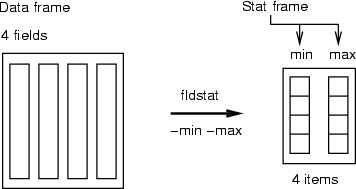
| fldstat | Macro command for computing statistics for fields |
| -d <srcdata> | source data frame |
| -dout <trgdata> | target data for statistics in classes |
| [-min] | find minimum values |
| [-max] | find maximum values |
| [-sum] | compute sum values |
| [-avg] | compute average values |
| [-var] | compute variances |
| [-dev] | compute standard deviations |
| [-md <value>] | missing value to be skipped |
| [-sw <field>] | sampling weights field |
This is a macro command, which includes the commands listed in the following section. Each operation stores results in one field meaning that, for instance, all minimum values from the data fields will be stored in one field. New fields, which are created into <trgdata>, are named with the name of the operation performed (min, max, sum, avg, ...). Missing values and sampling weights are explained in detail in Section 4.7.1.
| fldmin | Find the minimum values of the fields |
| -d <srcdata> | source data frame |
| -fout <trg-field> | field to be created |
| [-dout <trgdata>] | target data for statistics in classes |
| [-md <value>] | missing value to be skipped |
| fldmax | Find the maximum values of the fields |
| -d <srcdata> | source data frame |
| -fout <trg-field> | field to be created |
| [-dout <trgdata>] | target data for statistics in classes |
| [-md <value>] | missing value to be skipped |
| fldavg | Compute the average values of the fields |
| -d <srcdata> | source data frame |
| -fout <trg-field> | field to be created |
| [-dout <trgdata>] | target data for statistics in classes |
| [-md <value>] | missing value to be skipped |
| [-sw <field>] | sampling weights field |
| fldsum | Compute the sum values of the fields |
| -d <srcdata> | source data frame |
| -fout <trg-field> | field to be created |
| [-dout <trgdata>] | target data for statistics in classes |
| [-md <value>] | missing value to be skipped |
| [-sw <field>] | sampling weights field |
| fldvar | Compute the variances of the fields |
| -d <srcdata> | source data frame |
| -fout <trg-field> | field to be created |
| [-dout <trgdata>] | target data for statistics in classes |
| [-md <value>] | missing value to be skipped |
| [-sw <field>] | sampling weights field |
| flddev | Compute the standard deviations of the fields |
| -d <srcdata> | source data frame |
| -fout <trg-field> | field to be created |
| [-dout <trgdata>] | target data for statistics in classes |
| [-md <value>] | missing value to be skipped |
| [-sw <field>] | sampling weights field |
The field statistics compute statistical values from fields. These commands reduce the information of each field to one quantity, which is stored in a given field. If the output data frame has been specified, then the operation creates a data frame (if it does not exist) and adds the field into it. Otherwise, the new field is created directly into specified (or current) directory.
The form of the result is a column matrix in which one statistical value over all the fields is stored in one field. Each data record corresponds to a field in the source data. This differs from the class statistics in which data records correspond to original classes.
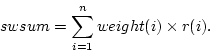
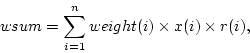
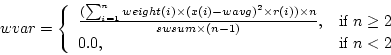
Each operation may take a missing value as a parameter. If the parameter is specified, then the defined value is skipped while computing the statistics. The effect of sampling weights for each statistical descriptor is explained in the following paragraphs.
Weighted sample average is calculated as
REMARKS:
Weighted sample sum is calculated as
Weighted sample variance is calculated as
Weighted sample deviance is square root of weighted sample variance, thus
Example (ex4.7): A typical use of field statistics is to compute minimum and maximum values or average and deviation from a frame for some scaling task.
...
NDA> fldstat -d boston -dout mmstat -min -max
NDA> ls -fr mmstat
 mmstat.min
 mmstat.max
NDA> fldstat -d boston -dout adstat -avg -dev
NDA> ls -fr adstat
 adstat.avg
 adstat.dev
| fldquar | Compute quatiles for data fields |
| -d <data> | source data |
| -fout <field> | resulted field |
| [-v <value>] | percentual amount of data |
| [-md <mvalue>] | missing value to be skipped |
| [-sw <field>] | sampling weights field |
This operation finds a value of the sorted data that limits a given portion of data. If <value> is not given, then the default value (50 %) is used.
Sample ![]() quartile, where
quartile, where ![]() , is solved as follows. First observed data values are sorted from lowest to highest values yielding into sorted indices
, is solved as follows. First observed data values are sorted from lowest to highest values yielding into sorted indices
![]() , where
, where ![]() is number of missing data values. Then the quartile is
is number of missing data values. Then the quartile is ![]() :th sorted observed data value, where
:th sorted observed data value, where ![]() is minimum index for which holds
is minimum index for which holds
Example: This simple example shows, how the first and the third quartiles can be computed.
NDA> load boston.dat
NDA> mkgrp grp
NDA> addsg grp
NDA> select crim -f boston.crim
NDA> fldquar -d crim -fout crim25 -v 25
NDA> fldquar -d crim -fout crim75 -v 75
NDA> rngplt grp -n crim -inx 0 -f crim25 -f crim75
     -sca data -min boston.crim -max boston.crim -co blue -labs
| fldhisto | Compute a histogram for a field |
| -f <field> | source field |
| -max <pins> | number of the pins |
| -dout <trgdata> | target data for a histogram |
| [-cum] | cumulative histogram |
| [-bounds] | save bounds of each pin into fields |
This operation computes a histogram for a field. The range of the field is divided into the specified number (<pins>) of uniform pins. Then the amount of hits is computed. The result will be a frame with two fields: x containing the centroids of the pins and N including the number of hits in pins. If -bounds is specified, two additional fields are inserted into the frame: low and up, which contain the lower and upper limits for each pin.
Example (ex4.8): This simple example shows, how a histogram can be computed for fuzzy coding. See also command hst (section 8.4.7) and the graphics part of this guide.
NDA> load boston.dat
NDA> mkfz fz
NDA> fldhisto -f boston.age -max 50 -dout hst
NDA> hst fz.grp -inx 0 -d hst.N -co red
NDA> addfzs fz -fs s1 -t 8
NDA> addfzs fz -fs s2 -t 8
NDA> initfz fz -lock
NDA> func1 fz.grp -f fz.sets.s1 -co blue
NDA> func1 fz.grp -f fz.sets.s2 -co blue
NDA> viewp fz.grp -dz 120
NDA> wrps -n fz.grp -o fzhst.ps -w 500 -h 200
| cmpquar | Compute a histogram for a field |
| -d1 <base-data> | base data |
| -d2 <data> | data to be compared |
| -dout <trgdata> | target data for portions |
This operation compares the specified <data> with <base-data> and replaces each value by perceptual portions that describe, how big part of the values of <base-data> is less than that particular value. The data frames are compared field by field.
Operations for computing class statistics follow the same principles as field statistics. An operation takes a classified data as a parameter. Then it collects all the data records pointed to by these classes and computes statistical values for them. The result will be a data frame, in which each class will have a data record and one statistical value over all classes is stored in a field. The principle of these operations has been described in the following figure:
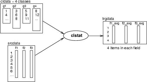
| clstat | Macro command for computing statistics for classes |
| -c <cldata> | classified data for defining classes |
| -d <srcdata> | source data frame |
| -dout <trgdata> | target data for statistics in classes |
| [-all] | compute all the statistics (other flags) |
| [-sum] | compute sums |
| [-avg] | compute averages |
| [-med] | compute medians |
| [-var] | compute variances |
| [-adev] | compute average |
| [-min] | find minimum values |
| [-max] | find maximum values |
| [-quar] | compute the first and the third quartiles (25%, 75%) |
| [-hits] | create a variable for the number of the items in classes |
| [-name] | the name of the class as a string |
| [-id] | the identifier of the class as an integer |
| [-md <value>] | missing value to be skipped |
| [-sw <field>] | sampling weights field |
This macro command computes statistics for classes of classified data <cldata> from <srcdata>. The procedures called by this command are documented in their own sections below. See fldsum (Section 4.7.1) for details on sampling weights. REMARK: -adev does not support sampling weights yet.
Example (ex4.9): In the first example, Boston data is classified between unique values located in field chas, which has two possible values: the appartment is located near the river (1) or not (0). Then the average values are computed from other fields. Also the numbers of items in both classes is evaluated.
...
NDA> select key1 -f boston.chas
NDA> uniq -d key1 -cout cld1
NDA> clstat -d boston -c cld1 -dout sta -avg -hits
NDA> ls -fr sta -f
 hits
 crim_avg
 zn_avg
...
Example (ex4.10): This second example demonstrates computing statistics for SOM neurons. One advantage of using the statistical values compared to the use of weights is, that they have clear interpretations such as mean, minimum and maximum of the data records chosen to the neurons.
...
NDA> somtr -d predata -sout som1 -l 4
...
NDA> somcl -d predata -s som1 -cout cld1
NDA> clstat -d boston -c cld1 -dout sta -all
| clsum | Compute sums for classes |
| -c <cldata> | classified data for defining classes |
| -d <srcdata> | source data frame |
| -dout <trgdata> | target data for statistics in classes |
| [-ext <extension>] | extension for the name of the class variable |
| [-md <value>] | missing value to be skipped |
| clavg | Compute averages for classes |
| -c <cldata> | classified data for defining classes |
| -d <srcdata> | source data frame |
| -dout <trgdata> | target data for statistics in classes |
| [-ext <extension>] | extension for the name of the class variable |
| [-md <value>] | missing value to be skipped |
| clvar | Compute variances for classes |
| -c <cldata> | classified data for defining classes |
| -d <srcdata> | source data frame |
| -dout <trgdata> | target data for statistics in classes |
| [-ext <extension>] | extension for the name of the class variable |
| [-md <value>] | missing value to be skipped |
| clmin | Find minimum values for classes |
| -c <cldata> | classified data for defining classes |
| -d <srcdata> | source data frame |
| -dout <trgdata> | target data for statistics in classes |
| [-ext <extension>] | extension for the name of the class variable |
| [-md <value>] | missing value to be skipped |
| clmax | Find maximum values for classes |
| -c <cldata> | classified data for defining classes |
| -d <srcdata> | source data frame |
| -dout <trgdata> | target data for statistics in classes |
| [-ext <extension>] | extension for the name of the class variable |
| [-md <value>] | missing value to be skipped |
This set of commands computes statistics for the classes of <cldata>, which refer to data records in <srcdata>. The checking of the context between the classes and data records of the source data is left to the user.
The macro command clstat and the separate commands can be used to compute the same statistics. The macro command also provides names to the fields of resulting data automatically by using extensions which correspond to actual procedures (_avg, _min, _max, etc.).
| clname | Create a field for the names of the classes |
| -c <cldata> | classified data for defining classes |
| -fout <field> | target field |
| -dout <trgdata> | target data for statistics in classes |
| [-id] | this flag causes to identify by integers |
This operation creates a name field, to which it generates the names of the classes. If the flag -id has been given, then identifiers are stored as integers. Otherwise they are stored as strings.
| clkey | Pick the first items of the classes |
| -c <cldata> | classified data for defining classes |
| -d <srcdata> | source data frame |
| -dout <trgdata> | target data for keys of classes |
| [-ext <extension>] | extension for the name of the class variable |
| [-md <value>] | missing value to be skipped |
This command picks one value from each field of source data for each class in the specified classified data. The values are stored to the given data frame in which one data record will correspond to one class.
| clhits | Evaluate the number of items in classes |
| -c <cldata> | classified data for defining classes |
| -fout <field> | target fields |
| [-dout <trgdata>] | target data for statistics in classes |
This command reads the sizes of the classes and creates a new data field to which these values are stored. Thus, one row in this field will correspond to one class.
| clquar | Computing quartiles for classes |
| -c <cldata> | classified data for defining classes |
| -d <srcdata> | source data |
| -dout <trgdata> | target data for statistics in classes |
| [-v <portion>] | the perceptual portion of the data (default 50%) |
| [-ext <extension>] | the extension for variables |
| [-md <value>] | missing value to be skipped |
This operation finds values in fields so that the given portion of the data will be left within the values. The procedure is performed for each field separately and results are stored with the names of the fields specified with an extension.
| cladev | Computing deviations |
| -c <cldata> | classified data for defining classes |
| -d <srcdata> | source data |
| -dout <trgdata> | target data for statistics in classes |
| -ext1 <ext1> | the extension for the variable |
| -ext2 <ext2> | the extension for the variable |
| [-md <value>] | missing value to be skipped |
The operation computes the values average ![]() deviation which will be stored with the extensions _ext1 and _ext2.
deviation which will be stored with the extensions _ext1 and _ext2.
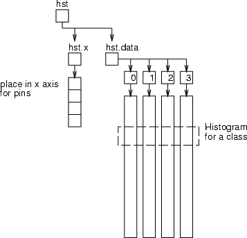
| clhisto | Computing histograms for classes |
| -c <cldata> | classified data for defining classes |
| -f <field> | source field |
| -dout <trgdata> | target data for statistics in classes |
| [-max <num-categ>] | the number of the categories (default 2) |
This operation computes histograms for a given field in the classes defined by <cldata>. The result will be a frame presented in the figure below. The frame hst has the field hst.x containing places for pins in the ![]() -axis and data frame hst.data to store actual fields for pins. One class is represented as one data record.
-axis and data frame hst.data to store actual fields for pins. One class is represented as one data record.
The commands introduced in this section are meant for specifying fuzzy sets and encoding data fields into fuzzy values. Typically the fuzzy commands have been hidden behind the GUI, but if you are developing a new user interface, then you should be familier with the commands, too.
The fuzzy tool operates with a fuzzy frame which includes membership functions and statistics and a graphic structure for the fuzzy tool as the following figure shows.
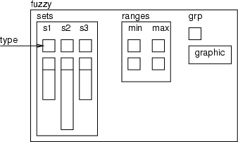
The fuzzy frame contains three parts: a frame for membership functions, a frame for the ![]() values and a graphic structure. The membership functions are handled as data fields in which the first value defines the type of the set and other values are function specific. The frame ranges includes the minimum and maximum values for fuzzy sets if the automatic initialization is used.
values and a graphic structure. The membership functions are handled as data fields in which the first value defines the type of the set and other values are function specific. The frame ranges includes the minimum and maximum values for fuzzy sets if the automatic initialization is used.
| mkfz | Create a fuzzy structure |
| <fuzzyname> | name of the fuzzy structure |
| [-f <field>] | name of a data field |
This command creates the fuzzy structure presented above. The frame sets is initialized to be empty. If a field is given, then the minimum and maximum values are located; otherwise they are set to 0.0 and 1.0. Also a graphic structure is created with one subgraph.
| addfzs | Add a new fuzzy set |
| <fuzzyname> | name of the fuzzy structure |
| -fs <setname> | name of the new set |
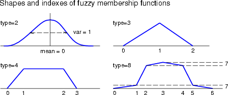
| -t <type> | 2 = gauss, 3 = triangular, 4 = trapezoidal, 8 = smoothed trapezoidal |
This command creates a new fuzzy set meaning that a new field with a given <type> is created to the frame sets under the fuzzy frame <fuzzyname>.
Example: The following command sequence demonstrates working with a fuzzy structure.
NDA> load boston.dat
NDA> mkfz fz1 -f boston.dis
# Add a fuzzy set for apartments near the city
NDA> addfzs fz1 -fs nearToCity -t 8
# Add a fuzzy set for apartments far from the city
NDA> addfzs fz1 -fs farFromCity -t 8
| initfz | Initialize fuzzy functions |
| <fuzzyname> | name of the fuzzy structure |
| [-fs <setname>] | name of the target set |
| [-lock] | locking similar sets to each other |
| setfzs | Macro to update a membership function of a fuzzy set |
| <fuzzyname> | name of the fuzzy structure |
| -fs <setname> | name of the fuzzy set |
| -vals <index>=<value> ...; | indexed point values ended with ';' |
| [-lock] | locking similar sets to each other |
| getfzpnt | Find the nearest point of the membership functions |
| <fuzzyname> | name of the fuzzy structure |
| -v <value> | the value to be located |
| [-lock] | check only suitable points for locked sets |
These commands are meant for setting or getting the shapes of membership functions. The membership functions are specified through the names of the fuzzy sets, the indexes of the corner points or values of these corners in the x-axis. The indexes for each type of fuzzy membership function are illustrated in the figure below. If the parameter -lock has been given for these commands, then the sets are handled as if they were locked to each other. getfzpnt can be used to find the nearest point among suitable points.
Example: This example demonstrates commands which are needed to create a drag-and-drop functionality to an interface for updating the access points of membership functions.
NDA> load boston.dat
NDA> mkfz fz1 -f boston.dis
NDA> addfzs fz1 -fs nearToCity -t 8
NDA> addfzs fz1 -fs farFromCity -t 8
NDA> initfz fz1
...
# Drag started at x-value 8.0, so find the nearest point of
# current membership function for location 8.0
NDA> getfzpnt fz1 -v 8.0
8.460867                 # The exact value of the point
nearToCity               # Set name
4                        # Index
...
# Create here drag-and-drop graphical output and, when the drop
# event is received, perform the following command:
NDA> setfzs fz1 -fs nearToCity -v 4=<x_value_for_drop>;
...
The example (ex4.11) demonstrates how a fuzzy structure and sets can be managed with a few commands. The fuzzy tool only includes the commands needed to modify fuzzy set structures. Therefore, you must also use operations modifying graphic structures, if you would like to support working with fuzzy sets using a graphical interface. Typically the fuzzy tool should hide these commands and thus only developers need to become familiar with them.
# Example: fuzzy sets
NDA> load boston.dat
NDA> mkfz fz1 -f boston.dis
# Set a histogram
NDA> rm -ref fz1.ranges
NDA> select ranges -f boston.dis
NDA> fldstat -d ranges -dout fz1.ranges -min -max
NDA> saxis fz1.grp -ax x -inx 0 -sca data -min fz1.ranges.min
 -max fz1.ranges.max -step 10
NDA> fldhisto -f boston.zn -max 50 -dout hst
NDA> hst fz1.grp -inx 0 -d hst.N -co red
# Add a fuzzy set for appartments near the city
NDA> addfzs fz1 -fs nearToCity -t 8
NDA> initfz fz1 -fs nearToCity -lock
NDA> func1 fz1.grp -inx 0 -f fz1.sets.nearToCity -co blue
NDA> updgr fz1.grp func1
# Add a fuzzy set for appartments far from the city
NDA> addfzs fz1 -fs farFromCity -t 8
NDA> initfz fz1 -fs farFromCity -lock
NDA> func1 fz1.grp -inx 0 -f fz1.sets.farFromCity -co blue
NDA> updgr fz1.grp func1
NDA> setimg fz1.grp -t vec
NDA> showfz fz1
| calcfz | compute membership values for a field |
| <fuzzyname> | the name of the fuzzy |
| -f <field> | field to be fuzzified |
| -dout <dataout> | result data frame |
This command computes membership values for a field. It creates a new field for each fuzzy sets. Then the membership values related to each set are computed. The names of the new fields will be the same as the names of the fuzzy sets.
From data records to data records
This command can be used to calculate a new data frame containing distances from a group of data records of one frame to another group of data records of another (or the same) frame. The distance measure can be a) euclidean, b) Hamming or c) Levenshtein distance. The result is a new data frame containing fields with names `0', `1', `2' and so on. These names indicate the data record indices of the first group, and data record numbers are the indices of data records in the second group.
Euclidean distance is calculated normally with
![]() . Hamming distance performs a comparison of data records and the resulting distance indicates the number of field values, in which they differ. When Hamming distance is used, the original data frames may contain STRING fields. In that case the distance indicates the number of character positions that are different in the evaluated strings. Levenshtein or EDIT distance locates the minimum number of character addition, deletion or update operations required to change the string in the first frame into a string in the second frame. In this case a single field name needs to be specified. The same field must be available in both original frames and it must be of type STRING.
. Hamming distance performs a comparison of data records and the resulting distance indicates the number of field values, in which they differ. When Hamming distance is used, the original data frames may contain STRING fields. In that case the distance indicates the number of character positions that are different in the evaluated strings. Levenshtein or EDIT distance locates the minimum number of character addition, deletion or update operations required to change the string in the first frame into a string in the second frame. In this case a single field name needs to be specified. The same field must be available in both original frames and it must be of type STRING.
Subsets of original data records can be specified using classes <class1> and <class2>. Omission of <class1> (and <class2>) results in the evaluation of all data records. If <data2> is not specified, <data1> is used instead. Minimum, maximum and average distances can be calculated and stored using switches -dmin, -dmax and -davg. All results are FLOATs for euclidean distance and INTs otherwise.
| dist | Calculate euclidean, Hamming or Levenshtein distances between data records |
| -d1 <data1> | name of the first original data frame |
| -dout <dataout> | distances between data vectors |
| [-cl1 <class1>] | name of the first class specification |
| [-d2 <data2>] | name of the second original data frame |
| [-cl2 <class2>] | name of the second class |
| [-dmin <do-min>] | field name for located minimum distance |
| [-dmax <do-max>] | field name for maximum distance |
| [-davg <do-avg>] | field name for average distance |
| [-ham] | calculate Hamming diatance instead of euclidean |
| [-lev <lev-fld>] | calculate Levenshtein (or EDIT) distance for specified field |
This command creates new fields to a data frame containing distances from some data vectors to some other data vectors within the same or different data sets. Distance measure can be euclidean, Hamming or Levenshtein. Located minimum, average and maximum distances can be stored for later use.
Example: Following commands calculate: a) euclidean distance between all data records of data1 and data2, b) Hamming distance between data3 and data4 and c) Levenshtein distance between data3.str and data4.str.
# List the contents of name space
NDA> ls -l -fr
 fr  d   /data1
 int f   /data1.x
 flt f   /data1.y
 fr  d   /data2
 int f   /data2.x
 flt f   /data2.y
 fr  d   /data3
 int f   /data3.x
 flt f   /data3.y
 str f   /data3.str
 fr  d   /data4
 int f   /data4.x
 flt f   /data4.y
 str f   /data4.str
# Calculate distances from data records to others
NDA> dist -d1 data1 -d2 data2 -dout dists1
NDA> dist -d1 data3 -d2 data4 -dout dists2 -ham
NDA> dist -d1 data3 -d2 data4 -dout dists3 -lev str
Calculation of euclidean distance between data3 and data4 would result in an error message:
NDA> dist -d1 data3 -d2 data4 -dout dists
 Returned error -450: Type does not match
From data records to group representatives
This command can be used to calculate a new data frame containing distances from all data records of a frame to several groups identified by a classified data. The distance can be measured as a) single linkage or b) group-average linkage (see figure below). Single linkage method locates the closest group member, and group-average first evaluates the average point for each group and calculates the distances between these group-averages and all data records. The result is a new data frame containing fields having the names of the groups identified in the classified data.
The calculation complexity of group-average linkage can be much smaller, but it cannot be used with certain types of data distributions. Part c) of the following figure depicts a problematic data distribution for group-average linkage.
There is also a local distance model available, in which all distances are limited to located minimum group-to-group distances. These minimum group distances are evaluated using single or group-average linkage according to chosen method.
| cldist | Calculate euclidean distances between data records and groups |
| -d <datain> | name of the original data to be used |
| -c <cldata> | classified data containing groupings |
| -dout <dataout> | distances from each vector to groups |
| [-dmax <maxfld>] | field name to use for maximum distance |
| [-gavg] | group-average linkage instead of single |
| [-local] | use locally limited distances |
This command creates new fields to a data frame containing distances from data vectors to groups of data vectors within the same data set. The groupings are identified by a classified data structure. The fields in output data are named according to group names. Located maximum distance can be stored for later use.
Example: For an example, see grpms (section 4.11).
This command is used for the evaluation of group memberships. Some type of dissimilarity measures, in which a value of 0 means that some data record is quite similar to some other, for example group representative, and a large value means that the data record is really different, can be converted into group memberships between 0.0 (really far from the group) and 1.0 (belongs to the group).
To evaluate these memberships, the maximum dissimilarity (or distance) for each original field is located (if it has not been specified on the command line). Normal distance calculation results in a global decrease of the group membership within the data distribution. However, the local mode of distance calculation results in a data, in which group membership decreases to 0.0 before closest group boundary or average is reached. All dissimilarity values larger than a specified one result in a membership of 0.0.
There are several membership functions that can be used. Default is linear, but negative exponential functions (
![]() ,
, ![]() ,
, ![]() , ...) and logistic sigmoid (
, ...) and logistic sigmoid (
![]() ) can also be used.
) can also be used.
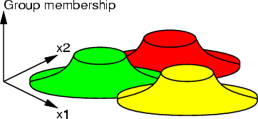
The following figure illustrates a two-dimensional case with three groups. The distances ![]() have been calculated with the single linkage local model and group averages have been evaluated with a second-order negative exponential function.
have been calculated with the single linkage local model and group averages have been evaluated with a second-order negative exponential function.
| grpms | Evaluate group memberships according to dissimilarity |
| -d <datain> | dissimilarity measures for each group |
| -dout <dataout> | calculated group memberships |
| [-dmax <maxfld>] | name of field containing specified maximum dissimilarity |
| [-npow <exp>] | decrease according to a <exp>-order negative exponential function (default linear) |
| [-logsig] | decrease according to a logistic sigmoid |
| [-scale] | divide all memberships by located maximum cumulative membership |
| [-scale1] | scale all cumulative memberships to 1.0 |
| [-limit1] | limit cumulative memberships to 1.0 |
| [-null] | set other group memberships to 0.0, if one is 1.0. Works only with -limit1 |
Command calculates group memberships according to dissimilarity (or distance) between a data vector and selected groups. Group memberships are scaled between 1.0 and 0.0 and decrease according to linear, negative exponential or logistic sigmoid function. For each group separately, maximum dissimilarity is located, if it has not been specified. Cumulative group memberships for each data record can be limited to 1.0, scaled to result a sum of 1.0 or scaled by dividing with located maximum sum.
Example: Following commands create a frame containing group memberships of a rule-based grouping. These memberships are based on euclidean distances between data vectors and the selected group centroids.
# Load a two-dimensional test data containing random points
#  within the square (0,0), (0,1), (1,0) and (1,1)
NDA> load testi.dat -n t
- field <x> (len 1)
- field <y> (len 1)
# Select groups: xL - x large & y small, yL - y large & x small
NDA> selcl -cout cldO -clout xL -expr 't.x'>=0.7 and 't.y'<=0.3;
NDA> selcl -cout cldO -clout yL -expr 't.y'>=0.7 and 't.x'<=0.3;
# Calc. distances from data records to group averages, local mode
NDA> cldist -c cldO -d t -dout Dist -gavg -local
# Evaluate group memberships according to the distances
NDA> grpms -d Dist -dout GrpMs -logsig
NDA> ls -fr GrpMs
 GrpMs.xL
 GrpMs.yL
If the group memberships of the example, xL and yL, are used as the z-axis of the original two-dimensional data and points are drawn into a window, the result is similar to the following figure. xL is denoted with red color.
| tfunc | Percentiles of the |
| -deg <n> | degrees of freedom |
| -val <value> | given percentage value |
| -fout <confidence> | name for the field with the level of confidence |
This function calculates the percentiles of the ![]() -distribution or the level of confidence for the given value with
-distribution or the level of confidence for the given value with ![]() degrees of freedom.
degrees of freedom.
Example: This example demonstrates the percentile of ![]() -distribution calculation.
-distribution calculation.
NDA> tfunc -deg 1 -val 1 -fout confidence
NDA> getdata confidence -tab
0.75
NDA> tfunc -deg 1 -val -1 -fout confidence2
NDA> getdata confidence2 -tab
0.25
| tinv | Inverse of the |
| -deg <n> | degrees of freedom |
| -conf <confidence> | given level of confidence |
| -fout <inverse> | name for the field with the inverse value |
This function calculates the inverse of the ![]() -distribution function by the given level of confidence with
-distribution function by the given level of confidence with ![]() degress of freedom.
degress of freedom.
Example: This example demonstrates the inverse of ![]() -distribution.
-distribution.
NDA> tinv -deg 1 -conf 0.75 -fout value
NDA> getdata value -tab
1
NDA> tinv -deg 1 -conf 0.25 -fout value2
NDA> getdata value2 -tab
-1
| fdist | |
| -val <value> | value |
| -n1 <n1> | first degrees of freedom |
| -n2 <n2> | second degrees of freedom |
| -fout <result> | name for the field with the result value |
| [-inv ] | switch for the inverse function |
If the switch -inv is not given this function calculates level of confidence of the standard ![]() -distribution function by the value given with the switch -val. Degrees of freedom given with the switches -n1 and -n2.
-distribution function by the value given with the switch -val. Degrees of freedom given with the switches -n1 and -n2.
If the switch -inv is given the function makes inverse operation, so the level of confidence must be given with the switch -val.
NDA> fdist -val 161.4 -n1 1 -n2 1 -fout result
NDA> getdata result -tab
0.95
NDA> fdist -val 0.95 -n1 120 -n2 120 -fout result -inv
NDA> getdata result -tab
1.35
| normalconf | uncdf |
| -value <value> | value |
| -fout <result> | name for the field with the result value |
The function normalconf calculates the value of the standard univariate normal cumulative function in the point given with the -value.
Thus it calculates the integral
| normalvalue | Inverse of uncdf |
| -conf <conf> | confidence |
| -fout <result> | name for the field with the result value |
The function normalvalue calculates the inverse of the standard univariate normal cumulative function. The quantity of the integral
![]() is given with the switch -conf. The result value will be in the field given with the switch -fout.
is given with the switch -conf. The result value will be in the field given with the switch -fout.
NDA> normalconf -value 0 -fout result
NDA> getdata result -tab
0.5
NDA> normalvalue -conf 0.5 -fout vresult
NDA> getdata vresult -tab
0.0
| mvncdf | Multivariate normal cumulative distr. function |
| -d <cov> | The covariance matrix |
| -dout <result> | The result frame |
| -f1 <low> | The field with the mean values |
| -f2 <low> | The field with the lower bounds |
| -f3 <up> | The field with the upper bounds |
| [-max <max>] | Maximum number of interations, default 300 |
| [-err <maxerr>] | Error value, default 0.01 |
| [-conf <conf>] | Confidence value, default 95.0 |
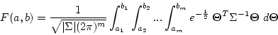
The function mvncdf calculates the multivariate normal cumulative distribution function. Hence, it calculates the integral
With the switch -d the user have to give the frame with the positive definite covariance matrix of the variables ![]() . The field -f1 must contain the vector with mean values
. The field -f1 must contain the vector with mean values
![]() . The fields -f2 and -f3 contain the vectors with lower and upper boundaries
. The fields -f2 and -f3 contain the vectors with lower and upper boundaries
![]() and
and
![]() .
.
The number of iteration is given with the switch -max. The calculated quantity of the integral will be less then given error -err with certain level of confidence -conf. The result will be in the output frame given with the switch -dout.
NDA> mvncdf -d covariance -dout result -f1 means -f2 low -f3 up \
     -max 1000 -err 0.0001 -conf 99.9999
NDA> getdata result -tab
IntegralSum  Error    Iterations
0.191924     0.00003  569