Next: Basic computing operations Up: User's reference Previous: Basic operations for managing Contents

Subsections

Data reorganization

Data reorganization contains operations, with which a data can be arranged into a new format. They do not really create new data, but only reorganize the original data. There are three major cases:

Operations for arranging information in data frames
Operations for arranging information in classified data frames
Operations for arranging information in data frames related to classified data frames

Transposing a data frame

transpose Create transpose of a frame

-d <data> source data frame

-dout <dataout> target data frame

[-pre <prefix>] prefix for the names of created fields

This command creates a full transpose of a frame. Source frame fields become data records of the target data frame, in which fields are identified with names containing the prefix and the row number of the original data record within the source frame. The default prefix is `f'.

Example: In this example the source frame contains x, y and z coordinates of 150 data points, that is, each data record contains the coordinates of one single point. The resulting transpose koord contains only 3 data records. The first has the x coordinates of all the 150 points, second the y coordinates and third the z coordinates.

...
NDA> ls -fr points
 points.x
 points.y
 points.z
NDA> transpose -d points -dout koord -pre p
NDA> ls -fr koord
 koord.p1
 koord.p2
 koord.p3
...
 koord.p149
 koord.p150
NDA>

Joining data frames

join Fully join two data frames

-d1 <data1> source data 1

-d2 <data2> source data 2

-k1 <key1> keys corresponding to data 1

-k2 <key2> keys corresponding to data 2

-dout <dataout> target data

ijoin Join only the first occurrences

-d1 <data1> source data 1

-d2 <data2> source data 2

-k1 <key1> keys corresponding to data 1

-k2 <key2> keys corresponding to data 2

-dout <dataout> target data

These two commands perform joining operations. The first operation makes a full join, and the second operation picks only the first pair of the keys which match the joining.

Example: These commands are useful when a data has a relational form, where clear `index' keys of the data records can be found. In such a case, the analysis can be made by using the following concept. If we have a data, which tells who has bought which product(s), and we want to profile customers, which are identified by their codes. The first data records can be summarized according to the customer code, for instance, by computing the average value of some fields for each customer. Then the calculated values can be added into the original order frame using join and previously located unique customer keys (see the baseball example).

...
NDA> ls -fr orderData
 custNro
 custSize
 custCover
# Summarize the data related to the customer number (custNro)
NDA> select keyFr -f orderData.custNro
NDA> uniq -d keyFr -cout custUniqs
NDA> select custFlds -f orderData.custSize orderData.custCover
NDA> clstat -d custFlds -c custUniqs -dout custData -avg
...
# SOM analysis -> groups of neurons
#              -> binarize them into data2
...
# Bind the customer key to data2 by the key operation
NDA> select custKeyOrg -f orderData.custNro
NDA> clkey -d custKeyOrg -c custUniqs -dout custData
NDA> select custKey -f custData.custNro
...
# Join binarized groups to the original data
NDA> cd ..
NDA> join -k1 keyFr -d1 orderData -k2 custKey 
     -d custData -dout data2

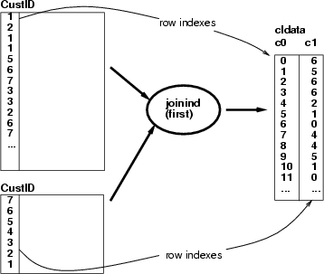
Indexing through a joining operation

joinind Store indexes from a joining operation

-k1 <key1> keys corresponding to data 1

-k2 <key2> keys corresponding to data 2

-cout <cldataout> target data

[-first] only the first matching pair is picked

[-full] classifying by the full joining

This operation creates a classified data frame containing the indexing for the results of a joining operation. The operation has two alternatives, how to create the classified data:

With the flag -full:

All data records in the first frame <key1> will have their own classes, in which the indexes refer to the matching data records in <key2>. Searching is performed over all records in both data frames. The classes are named with a running index beginning from `0'.

$\begin{figure}\centerline{\hbox{ \psfig{figure=joinind2.ps,width=10cm} }} \end{figure}$

Without the flag -full:

The joining operation finds the matching records and stores their indexes into two data fields. If the flag -first has been given, then only the first matching pair is picked for each record in data frame <key1>. The result is a classified data containing two classes with the same length. The first class is a running index to <key1> and the second class contains the indexes of the first matching records in <key2>. The names of the classes will be `0' and `1'.

$\begin{figure}\centerline{\hbox{ \psfig{figure=joinind1.ps,width=8cm} }} \end{figure}$

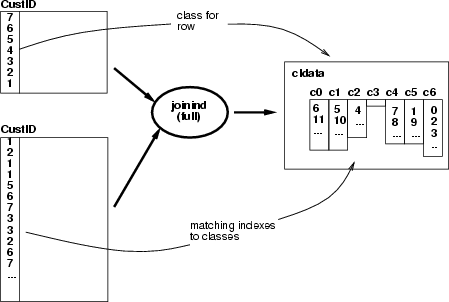
Example: SOM 1 has been trained with a data set describing baseball teams and SOM 2 with a data describing the players (hitters). The following script picks the identifiers of the teams from a selected neuron and finds all the players in those teams. Then all the neurons which include at least one of the team's players will be referred to by a classified data (see the baseball example).

...
# User has selected a neuron identified by $1
#
# 1. Pick teams and their identifiers from the select neuron
#
NDA> select neuronclass -cl grp.neuron_$1
NDA> pickrec -d teamKey -c neuronclass -dout selTeamKeys
#
# 2. Join teams to players based on teams' names and find their
#    identifiers. The names of the players are stored
#    in data frame /hitterTmp/hitterKey.
#
NDA> rm -fr /hitter/selHitterKey
NDA> join -k1 selTeamKeys -k2 /hitter/hitterTeamKey
     -d2 /hitter/hitterKey -dout /hitter/selHitterKey
#
# 3. The player names are mapped to a player data and matching
#    pairs are stored in a classified data /hitter/hitterRows
#    as (team_index, player_index) pairs.
#
NDA> joinind -k1 /hitter/selHitterKey -k2 /hitter/hitterKey
     -cout /hitter/hitterRows -first
#
# 4. Find neurons from the player SOM such that
#    it includes at least one player from the selected team
#
NDA> select /hitter/xxx -cl /hitter/hitterRows.1
# Select one layer from a SOM classification
NDA> somlayer -s  /hitter/som -f /hitter/somlayer
NDA> selcld -c /hitter/cld -expr '/hitterdir/somlayer'=2;
     -cout /hitter/layercld -empty
# Find the BMU for each indexes in /hitter/xxx (joined rows) and
# remove multiple indexes
NDA> findcl -c1 /hitter/layercld -c2 /hitter/xxx -cout /hitter/grp
NDA> uniqcl -c /hitter/grp -cout /hitter/groups
# The result /hitter/grp includes the indexes of the neurons
# that can be used as a group of the neurons.
...

Finding unique data records

uniq Choose unique data records into classes

-d <data> source data

-cout <cldata> target classification

[-auto] automated naming for classes

This operation locates unique data records. It creates a class for each unique key and collects the indexes of those data records matching the key into the class. If flag -auto is given, then the new classes are named using a running index. Otherwise, created new classes are named using the names of the fields and a combination of the values in those "unique" data records.

Example: A typical use for uniq is to find unique data records according to some key fields and then summarize other descriptive fields within these unique groups.

...
# Summarize Boston data according to boston.chas
NDA> select keyFr -f boston.chas
NDA> uniq -d keyFr -cout custCld
NDA> clstat -d boston -c custCld -dout custData -avg
...

Finding unique indexes from classes

uniqcl Find unique indexes from classes

-c <cldata> a source classified data

-cout <target> target classification

This operation locates unique indexes from classes of <cldata> and stores them in a similar classification. Classes in the <target> frame are named according to the source frame.

Some operations, such as findcl may refer to the same index several times in their resulting classified data. uniqcl can be used to eliminate indexes used in multiple occasions. This command has been used with joinind and findcl in the example of section 3.3.

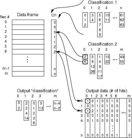
Finding the indexes of a classified data from another classified data

findcl Find the indexes of a classified data from another classified data

-c1 <cldata1> classified data for classes

-c2 <cldata2> classified data to be mapped

-cout <cldata> resulting classified data

[-first] locate only the first matching index

This operation matches the indexes of classified data <cldata2> to the indexes of classified data <cldata1>, and replaces indexes in <cldata2> with the indexes of that class of <cldata1>, from which the first occurrence or all occurences are found. The whole procedure is presented below, and a step for matching one index is described as a figure:

For each $index_{c2} \in cld2$
For each class $cl_i \in cld1$
For each $index_{c1} \in cl_i$
If $index_{c1} = index_{c2}$ Then
Add to $index_{trg}$ in the target classified data
Continue with next $index_{c2}$ if -first specified
EndIf
End
End
End

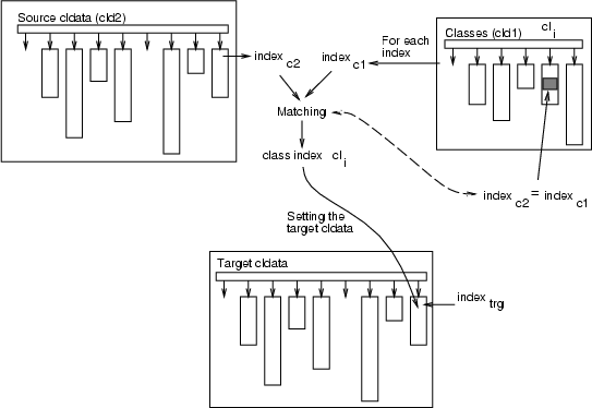
$\begin{figure}\centerline{\hbox{ \psfig{figure=findcl.ps,width=12cm} }} \end{figure}$

Example: See the example of joinind (section 3.3).

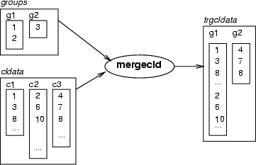
Merging a grouping and a classified data

mergecld Merge a classified data with groups

-c1 <groups> classified data for defining the groups of the classes in <cldata>

-c2 <cldata> classified data to be grouped

-cout <trgcldata> result classified data

This command merges classes of <cldata> according to the class groups defined in classified data <groups>. In this case, the identifiers in <groups> do not refer to actual data records. Instead, they refer to the classes in <cldata>. Resulting classes are named according to the classes in <groups>.

Example (ex3.1): In the case of SOMs, merging means that data records, which are divided between the neurons, are collected to larger classes. In other words, the indexes of the data records chosen to the neurons belonging to some neuron group are collected to the same class in the classified data trgcldata.

...
NDA> somtr -d boston -sout som1 -cout cld1 -l 4
...
NDA> mkgrp grp1 -s som1
...
# Grouping with a graphical tool -> groups are stored in the
# classified data "som1Grp". SOM classification for data records
# is stored in "cld1".
NDA> mergecld -c1 som1Grp -c2 cld1 -cout classif
# To utilize the classification "classif":
NDA> bin -d boston -c classif -dout data2
NDA> pickrec -d boston -c classif -dout data3

$\begin{figure}\centerline{\hbox{ \psfig{figure=mergecld.ps,width=8cm} }} \end{figure}$

Set-relational operations for classes

These set operations can be used to compare single classes or complete classifications having the same class names.

clinsec Evaluate the intersection of two classes

-cl1 <data1> source class 1

-cl2 <data2> source class 2

-clout <dataout> target class

clunion Evaluate the union of two classes

-cl1 <data1> source class 1

-cl2 <data2> source class 2

-clout <dataout> target class

cldiff Evaluate the difference of two classes

-cl1 <data1> source class 1

-cl2 <data2> source class 2

-clout <dataout> target class

These three commands perform normal set operations intersection, union or difference to two classified data classes. Intersection contains those data record indices included in both classes, union contains a superset of all indices within the two classes and difference those indices within just one of the classes, but not in both of them.

Example: For a thorough example, see the example of classification comparisons. Here is just a basic example with a small data set.

...
# Data file with 8 numbers (1, 2, 3, 5, 8, 6, 7 and 4)
NDA> getdata k
x                               # Field name
1                               # Data type (integer)
1                               # Data values
2
3
5
8
6
7
4
# Select two classes containing indices to values larger than
# or equal to 3 (first) and values between 5 and 7 (sec)
NDA> selcl -cout cli -clout first -expr 'k.x' >= 3;
NDA> selcl -cout cli -clout sec -expr 'k.x' >= 5 and 'k.x' <= 7;
# Evaluate difference of classes
NDA> cldiff -cl1 cli.first -cl2 cli.sec -clout cli.result
NDA> save cli
...

# This results in cli.cld containing the following data lines:
...
class_info
201 1 first 6 2 3 4 5 6 7 
201 1 sec 3 3 5 6 
201 1 result 3 7 4 2 
# Class first: 6 indices (234567), class sec 3 indices (356),
# Difference(result):  3 indices (247)

cldinsec Evaluate the intersection of two classifications

-c1 <cldata1> source classified data 1

-c2 <cldata2> source classified data 2

-cout <cldataout> target classified data

cldunion Evaluate the union of two classifications

-c1 <cldata1> source classified data 1

-c2 <cldata2> source classified data 2

-cout <cldataout> target classified data

clddiff Evaluate the difference of two classifications

-c1 <cldata1> source classified data 1

-c2 <cldata2> source classified data 2

-cout <cldataout> target classified data

These commands perform class by class set operations for entire classifications. Each class name of classified data <cldata1> is compared to the names of classes in <cldata2>. If a match is found, a new class with the same name is created into the target classified data containing the intersection, union or difference.

Example: To compare the classification results of two different layers of TS-SOM, union and intersection can be used.

...
# Data loaded into d - Selection of fields, training of a SOM
NDA> select datas -f d.GP d.GN d.TP d.TN
NDA> somtr -d datas -sout som -cout cldata -l 4
 Trained layer: 0
 Trained layer: 1
 Trained layer: 2
 Trained layer: 3
# Average value calculation for each neuron
NDA> clstat -c cldata -d datas -dout st -avg
NDA> ls -fr st
 st.GP_avg
 st.GN_avg
 st.TP_avg
 st.TN_avg
# TS-SOM layer info is needed for selection of data records
NDA> somlayer -s som -fout sl
NDA> selcl -cout g2 -clout GP -expr 'sl'=2 and 'st.GP_avg'>=0.7;
NDA> selcl -cout g2 -clout GN -expr 'sl'=2 and 'st.GN_avg'>=0.7;
NDA> selcl -cout g2 -clout TP -expr 'sl'=2 and 'st.TP_avg'>=0.7;
NDA> selcl -cout g2 -clout TN -expr 'sl'=2 and 'st.TN_avg'>=0.7;
NDA> selcl -cout g3 -clout GP -expr 'sl'=3 and 'st.GP_avg'>=0.7;
NDA> selcl -cout g3 -clout GN -expr 'sl'=3 and 'st.GN_avg'>=0.7;
NDA> selcl -cout g3 -clout TP -expr 'sl'=3 and 'st.TP_avg'>=0.7;
NDA> selcl -cout g3 -clout TN -expr 'sl'=3 and 'st.TN_avg'>=0.7;
# Selected groups of records need to be converted into cldatas
NDA> mergecld -c1 g2 -c2 cldata -cout clo2
NDA> mergecld -c1 g3 -c2 cldata -cout clo3
# Compute intersection and union of indices in classifications
NDA> cldinsec -c1 clo2 -c2 clo3 -cout clo_insec
NDA> cldunion -c1 clo2 -c2 clo3 -cout clo_union
# Calculate the index counts of each class into a frame
NDA> clhits -c clo_insec -fout ins
NDA> clhits -c clo_union -fout uni
NDA> select clp -f ins uni
NDA> ls -fr clp
 clp.ins
 clp.uni
# Calculate the ratio of the set sizes (intersection / union)
# for each class (GP, GN, TP and TN)
NDA> expr -dout props -fout prop -expr 'clp.ins' / 'clp.uni';
NDA> getdata props
prop
2
0.870521
0.940236
0.810526
0.972215
...

Convert a classification into a field

cldind Convert cldata into a field

-c <cldata> classified data to be converted

-d <data> original data frame

-fout <field> field to be created

This operation makes it possible to convert a classified data into a data field. The resulting data field contains the index of the class (ranging from 1 to , where is the number of classes), to which the record belongs. The conversion is complete only if each data record belongs to only one class. Otherwise each record gets the index of the last class, to which it belongs to.

Example: In this example a SOM classification is converted into a field to be used as training data for another SOM.

# Load training data set
NDA> load opetus
# Train a SOM and create field containing SOM layers
NDA> somtr -d opetus -sout som -cout cldata -l 7
...
NDA> somlayer -s som -fout soml
# Select the 6th layer of TS-SOM into a new cldata
NDA> selcld -c cldata -cout clsel -expr 'soml' = 6;
# Convert classification into a data field
NDA> cldind -c clsel -d opetus -fout opetus.somind

Converting SOM classification to location codes

loccode Generate location codes from a field containing neuron numbers

-f <infield> source field

-fout <outpref> prefix for output data field(s)

-l <layer> layer of the original SOM

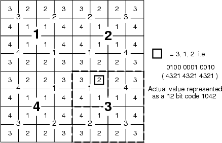
Generate a hierarchical location code from a data field containing SOM neuron classification numbers. Resulting codes indicate, into which quarter and subquarter and so on, data records have been captured. Each division into four parts increases the length of the code by four bits. Therefore, the codes are 24 bits for the 6th layer of TS-SOM, for example. There is only a single bit difference between codes of neighboring neurons. The code is packed into variables <outpref>_0, <outpref>_1, ... each containing 24 bits of information. The following figure illustrates the coding scheme using the third layer.

$\begin{figure}\centerline{\hbox{ \psfig{figure=loccode.ps,width=10cm} }} \end{figure}$

Example: See the example of lcode2bin.

lcode2bin Convert location codes into binary fields

-f <infield> source field prefix

-dout <frame> output data frame for binary fields

-bits <numbits> number of bits in location codes

[-grps <grpsize>] number of bits in each group

[-wght <residual>] residual to be used for neighbors of 1s

This command converts a "24 bits/variable" location code into binary variables, which are put into the output frame. The number of bits in the whole code needs to be specified and the number of input fields can be calculated from that. Input fields need to be named as <inpref>_0, <inpref>_1, and so on. It is possible to have an additional weighting for the neighboring 0 bits of 1s and, if group size is specified, the neighborhood is determined within each group.

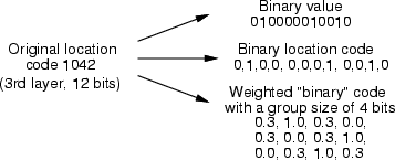
$\begin{figure}\centerline{\hbox{ \psfig{figure=lweight.ps,width=8cm} }} \end{figure}$

Example: If we have a SOM classification in cldata, the original data in frame tdat and TS-SOM layers in soml, with the following commands we can create a location code from the 6th layer into frame lbin and have a weighting of 0.3 for neighbors in each group of 4 bits.

# Select the classification of the 6th layer of TS-SOM
# into a new cldata
NDA> selcld -c cldata -cout clsel -expr 'soml' = 6;
# Convert classification into a data field
NDA> cldind -c clsel -d tdat -fout tdat.somind
# Create location codes for each neuron into tdat.lcds_0
NDA> loccode -f tdat.somind -fout tdat.lcds -l 6
# Convert these codes into a weighted "binary" frame lbin
NDA> lcode2bin -f tdat.lcds -dout lbin -bits 24 -grps 4 -wght 0.3

Combining classifications

clcomb Combine two classifications into one

-d <indata> original data frame

-c1 <cldata1> keys corresponding to the data 1

-c2 <cldata2> keys corresponding to the data 2

{-cout <cldataout> | combined classified data

-dout <dataout>} output data

[-lout <lossout>] output frame name for the number of unclassified records

[-bin] binary output instead of record counts

This operation combines two classifications into one. The resulting classes are created according to <cldata2>, but data record indexes are replaced with the class numbers of <cldata1>. If some data record that has been identified in <cldata2> does not belong to any class of <cldata1>, it is recorded in <lossout>, which is a frame containing the number of unclassified data records for each class of <cldata2>. The output data frame contains the number of data records belonging to a certain class of <cldata2> (field) and <cldata1> (record number). Binary output can be requested with -bin. Binary output merely indicates whether some feature of <cldata2> exists for a class of <cldata1>.

Example: To collect all neuron IDs, which have captured a certain group of data records, following commands can be issued:

# Load data and train a TS-SOM
NDA> load t.dat -n t
NDA> select opetus -d t
NDA> rm -fr opetus opetus.stid
NDA> rm -fr opetus opetus.exid
NDA> somtr -d opetus -sout som -cout cldata -l 6
...
NDA> somlayer -s som -fout soml
# Select two fields representing unique ID of groups of data
# records and create a classification, in which each class
# represents one group
NDA> select unifld -f t.stid t.exid
NDA> uniq -d unifld -cout unicld
# Select one layer of SOM classification
NDA> selcld -c cldata -cout cldl5 -expr 'soml' = 5;
NDA> clcomb -c1 unicld -c2 cldl5 -d t -dout hitcounts
# The resulting frame contains the number of data records
# having a certain combination of classifications
# Fields are named as neuron_...

$\begin{figure}\centerline{\hbox{ \psfig{figure=clcomb.ps,width=10cm} }} \end{figure}$

Converting sum values into propabilities

sums2prop Convert a frame of sum values into propabilities

-d <data> source data

-dout <trgdata> result data

This command converts a frame containing numerical values into propabilities by dividing each data record by the sum of its components.

Example: A frame of sums (see the example of clcomb, section 3.11) is converted into a frame of propabilities.

...
# Original data contains the number of hits
NDA> sums2prop -d hitcounts -dout hitprop
# Resulting data contains propabilities
# The sum of each data record is unity

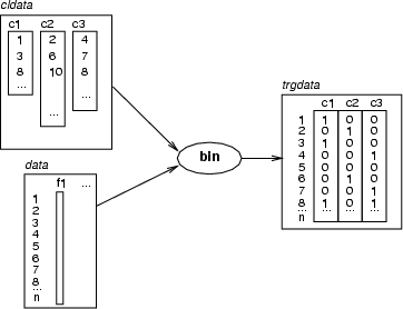
Binarizing a classification to data fields

bin Code classes in a classified data into binary variables

-c <cldata> classified data for identifying records

-d <data> source data

-dout <trgdata> result data

[-pre <prefix>] prefix for fields to be created

This command encodes a given classified data related to a source data. For each class a new binary (integer) field is created. Then, the index of each data record is matched to the indexes in the class. If the index is found, the value of the binary variable corresponding to that class will be `1', otherwise `0'. Target data can be the same as source data. In that case, new fields are created to the existing data frame. Otherwise, a new data frame is created. If <prefix> is specified, created fields are named as <prefix>_<n>, otherwise the names of the classes of <cldata> are used.

Example (ex3.3): This example shows necessary commands and phases needed to create a binary coding for a grouping of data.

...
NDA> somtr -d boston -sout som1 -l 4
...
NDA> somcl -d boston -s som1 -cout cld1
NDA> mkgrp grp1 -s som1
...
# Interactive selection of groups
NDA> mergecld -c1 som1Grp -c2 cld1 -cout classif
# Create a binary data according to selected groups
NDA> bin -d boston -c classif -dout data

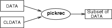
$\begin{figure}\centerline{\hbox{ \psfig{figure=bin.ps,width=8cm} }} \end{figure}$

Picking data records based on a classified data

pickrec Pick data records referenced by a classified data

-c <cldata> classified data for pointing records

-d <data> source data

-dout <trgdata> result data

This operation picks a subset of data records from <data>. The records to be picked are pointed to by the indexes in <cldata>. Typically this command is used to restrict the analysis scope to certain data records, which have been chosen to some neuron(s). With mergecld (see 3.7) such a classified data can be formed, which contains the indexes of data records chosen to several neurons.

Example (ex3.2): This example shows the necessary commands and phases needed to restrict scope to some part of the original data using a TS-SOM. select is used to select two groups g1 and g3, which could be analyzed in more detail in the second phase.

...
NDA> somtr -d boston -sout som1 -l 4
...
NDA> somcl -d boston -s som1 -cout cld1
NDA> mkgrp grp1 -s som1
...
# Interactive selection of groups
NDA> mergecld -c1 som1Grp -c2 cld1 -cout classif
# Select a subset of groups
NDA> select partCls -cl classif.g1 classif.g3
NDA> pickrec -d boston -c partCls -dout data3

$\begin{figure}\centerline{\hbox{ \psfig{figure=pickrec.ps,width=8cm} }} \end{figure}$

Sorting a data frame

sort Sort the records of a data frame

-k <keydata> key fields for sorting

-d <data> actual data fields to be sorted

-dout <trgdata> target data, which can also be the same as source data

[-desc] descending order

This operation sorts the given data frame, <data>, according to the keys in <keydata>. If result data is the same as <data>, then <data> is replaced with the sorted data. Otherwise, a new data frame is created.

Example (ex3.4): Here are two sorting examples for data frames.

...
# Ascending according to rate, replacing source with result
NDA> select key1 -f boston.rate
NDA> sort -k key1 -d boston -dout boston
# Two fields as keys, priorities: 1. dis, 2. rm
NDA> select key2 -f boston.dis boston.rm
NDA> sort -k key2 -d boston -dout boston2

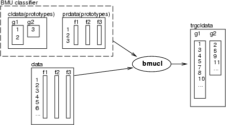
Classifying a data frame with a BMU classifier

bmucl Classify a data with a BMU classifier

-d1 <prdata> prototypes for classes

-c1 <cldata> classified data for collecting prototypes to classes

-d2 <data> data to be classified

-cout <trgcldata> result classified data

[-min <value>] Add <value> to all output indexes

This operation performs a B(est)M(atching)U(nit) classification. The classifier is defined by prototypes in <prdata> and a classified data that defines, which prototypes represent each class. The result will be stored in a new classified data <trgcldata>, in which classes will have the same names as in <cldata>. If <value> is specified, it is added to all indexes of the output classification.

Example (ex3.5): In the first example, four data records (4, 50 belonging to class c1 and 63, 150 to class c2) are selected to be prototypes of the classes. Then the same data, boston, is classified according to these prototypes.

...
NDA> addcld -c bmuclfr
NDA> addcl -c bmuclfr -cl c1
NDA> updcl -cl bmuclfr.c1 -id 4
NDA> updcl -cl bmuclfr.c1 -id 50
NDA> addcl -c bmuclfr -cl c2
NDA> updcl -cl bmuclfr.c2 -id 63
NDA> updcl -cl bmuclfr.c2 -id 150
NDA> bmucl -d1 boston -c1 bmuclfr -cout cld1

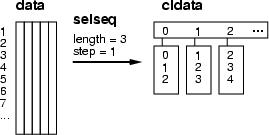
$\begin{figure}\centerline{\hbox{ \psfig{figure=bmucl.ps,width=10cm} }} \end{figure}$

Classifying data records to sequences

selseq Classify data records into sequences

-d <data> source data

-cout <cldata> target classified data

-len <lenght> the length of the sequence

[-step1 <step1>] step between time windows, default=1

[-step2 <step2>] step between data records within a time window, default=1

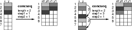
This operation creates a classified data frame and collects the indexes of data records to classes. The principle has been described in the figure below. As the figure shows, the operation moves a sliding window through a data frame collecting those data record indexes inside the window to the classes. The parameter <length> defines the length of the window. The parameter <step1> defines how many data records are skipped when the window is moved, whereas the parameter <step2> defines steps between data records. Of cource, then the true length of the time window is: <lenght> + (<length> 1) * <step2>.

$\begin{figure}\centerline{\hbox{ \psfig{figure=selseq.ps,width=6cm} }} \end{figure}$

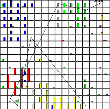
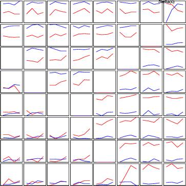
Example (ex3.6): This example demonstrates one way to process data including a code sequence. For instance, data includes codes 1, 9, 20, 2, 2, 3, 9, .... In the example, these codes are represented as binary variables (uniq and bin operations), and binary data is summarized over sequences (selseq and clsum).

NDA> load seq.dat
# Binarize code data
NDA> uniq -d seqdata -cout sequniq
NDA> bin -d seqdata -c sequniq -dout binseq
# Select sequences and summarize them
NDA> selseq -d binseq -cout seqcld -len 3
NDA> clsum -d binseq -c seqcld -dout binhst
# Basic SOM analysis for the sequence data
NDA> prepro -d binhst -dout pre -edev -n
NDA> somtr -d pre -sout som1 -l 5
...
NDA> somcl -d pre -s som1 -cout cld
NDA> clstat -d binhst -c cld -dout sta -avg -min -max -hits
# Create a graph
NDA> mkgrp win1 -s som1
NDA> setgdat win1 -d sta
NDA> setgcld win1 -c cld
NDA> layer win1 -l 4
# Show bars indicating different codes and a trajectory
NDA> bar win1 -f sta.code_0_avg -co red
NDA> bar win1 -f sta.code_6_avg -co green
NDA> bar win1 -f sta.code_8_avg -co blue
NDA> bar win1 -f sta.code_10_avg -co yellow
NDA> traj win1 -n tr1 -min 100 -max 110 -co black
NDA> show win1 -hide

$\begin{figure}\centerline{\hbox{ \psfig{figure=selseqres.ps,width=8cm} }} \end{figure}$

Concatenating sequences

concseq Concatenate data into sequences

-d <data> source data

-dout <dataout> target data

-len <lenght> the length of the sequence

[-c <cldata>] classified data for data record order

[-step1 <step1>] step between time windows, default=1

[-step2 <step2>] step between data records within a time window, default=1

[-empty] should partially empty sequences be created

This operation creates a new data frame, into which it concates data records from the given frame. The operation slides a window over the source data and concates data records falling within the window. If <cldata> has been defined, sequences are created according to the order provided by the classes. If -empty is not specified, all sequences for classes smaller than <lenght> are discarded.

For instance, if source data includes records $\{A_1,B_1\}$ , $\{A_2,B_2\}$ , $\{A_3,B_3\}$ , $\{A_4,B_4\}$ , and so on. If parameter <length> is 2 and <step1> is 1 (default), then target data will contain data records $\{A_1,B_1,A_2,B_2\}$ , $\{A_2,B_2,A_3,B_3\}$ , and so on. Here the indexes refer to the data records of source data. If parameter <step1> is specified, then the procedure skips over as many data records as defined, while moving the window. Parameter <step2> specifies the step between data records within the time window. See also the figure below and selseq (section 3.17).

The resulting data fields are named according to the names in source data with indexed extensions. The indexes are created to indicate the position inside the window. For instance, the field x would lead to new fields called x_0, x_1, x_2 and so on.

$\begin{figure}\centerline{\hbox{ \psfig{figure=concseq.ps,width=10cm} }} \end{figure}$

Example (ex3.7): The following example demonstrates the use of concseq. The length of the window is in this case four.

NDA> load gauss3.dat
# Collecting records
NDA> concseq -d gauss -dout gauss2 -len 4
# Normal SOM processing
NDA> prepro -d gauss2 -dout pre -edev -n
NDA> somtr -d pre -sout som1 -l 5
...
NDA> somcl -d pre -s som1 -cout cld
NDA> clstat -d gauss2 -c cld -dout sta -all
NDA> mkgrp win1 -s som1
NDA> setgdat win1 -d sta
NDA> setgcld win1 -c cld
NDA> show win1 -hide
# Visualization through line diagrams
NDA> ldgr win1 -n x -co red
NDA> ldgrc win1 -n x -inx 0 -f sta.x_0_avg -sca som2
NDA> ldgrc win1 -n x -inx 1 -f sta.x_1_avg -sca som2
NDA> ldgrc win1 -n x -inx 2 -f sta.x_2_avg -sca som2
NDA> ldgrc win1 -n x -inx 3 -f sta.x_3_avg -sca som2
NDA> ldgr win1 -n y -co blue
NDA> ldgrc win1 -n y -inx 0 -f sta.y_0_avg -sca som2
NDA> ldgrc win1 -n y -inx 1 -f sta.y_1_avg -sca som2
NDA> ldgrc win1 -n y -inx 2 -f sta.y_2_avg -sca som2
NDA> ldgrc win1 -n y -inx 3 -f sta.y_3_avg -sca som2
NDA> dis win1 ldgrlab
NDA> layer win1 -l 3
NDA> draw /win1

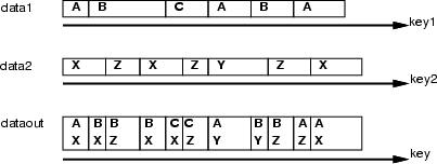
$\begin{figure}\centerline{\hbox{ \psfig{figure=concseqres.ps,width=8cm} }} \end{figure}$

Overlapping sequential data sets

mixseq Mix two event data sets

-k1 <time1> ordering keys for data 1

-d1 <data1> source data 1

-k2 <time2> ordering keys for data 2

-d2 <data2> source data 2

-dout <dataout> target data

This operation overlaps two event data sets <data1> and <data2> based on the orders defined through the corresponding key data sets <key1> and <key2>. The principle is presented in the figure below. mixseq assumes that the data sets have been ordered according to the key frame in ascending order. Then, it compares the "time" frames and collects mixed codes to the target frame. New fields in the target data are named using the names of data frames and fields (<data>_<field>). In addition, the operation creates a field called time to target data frame, into which the matched points are stored.

$\begin{figure}\centerline{\hbox{ \psfig{figure=mixseq.ps,width=9cm} }} \end{figure}$

Compacting self-similar data

compact Remove repeated data records to reveal trends

-d <datain> source data

-dout <dataout> target data

[-fout <recids>] original data record IDs, which were copied to target

This function removes repeating data records but preserves data record order. If certain data record is followed by another (or several) data record(s) that is (are) identical, these copies are not moved into the target data frame. The ID numbers of the original data frame that were copied to <dataout> are put into <recids>.

Example: A typical use of this command is to find unique instances of data without disturbing the order of events.

NDA> load process.dat -n data
# Select binary parameters representing process state
NDA> select statedata -f data.statep1 data.statep2 data.statep3
NDA> compact -d statedata -dout realstates -fout recids
# "realstates" could be used to train a SOM and visualize
# trajectories
# "recids" could be used to calculate statistics of other
# parameters for each distinct state

Changing field types

float2int Change float fields to integer fields inside frame

-d <datain> source data

int2float Change integer fields to float fields inside frame

-d <datain> source data

This is a raw operation. If there are other references to fields inside input frame these fields are changed too.

Example: In this example arbitary data containing float fields is loaded into memory and float fields inside the data frame are converted into integer fields.

NDA> load somedata.dat -n data
# Select some fields into other frame
NDA> select floatdata -f data.float1 data.float2
# Convert float fields inside data frame to integer.
NDA> float2int -d data
#  After this command "floatdata" contains only integer fields

Next: Basic computing operations Up: User's reference Previous: Basic operations for managing Contents

Anssi Lensu 2006-02-23

transpose	Create transpose of a frame
-d <data>	source data frame
-dout <dataout>	target data frame
[-pre <prefix>]	prefix for the names of created fields

join	Fully join two data frames
-d1 <data1>	source data 1
-d2 <data2>	source data 2
-k1 <key1>	keys corresponding to data 1
-k2 <key2>	keys corresponding to data 2
-dout <dataout>	target data
ijoin	Join only the first occurrences
-d1 <data1>	source data 1
-d2 <data2>	source data 2
-k1 <key1>	keys corresponding to data 1
-k2 <key2>	keys corresponding to data 2
-dout <dataout>	target data

joinind	Store indexes from a joining operation
-k1 <key1>	keys corresponding to data 1
-k2 <key2>	keys corresponding to data 2
-cout <cldataout>	target data
[-first]	only the first matching pair is picked
[-full]	classifying by the full joining

uniq	Choose unique data records into classes
-d <data>	source data
-cout <cldata>	target classification
[-auto]	automated naming for classes

uniqcl	Find unique indexes from classes
-c <cldata>	a source classified data
-cout <target>	target classification

findcl	Find the indexes of a classified data from another classified data
-c1 <cldata1>	classified data for classes
-c2 <cldata2>	classified data to be mapped
-cout <cldata>	resulting classified data
[-first]	locate only the first matching index

mergecld	Merge a classified data with groups
-c1 <groups>	classified data for defining the groups of the classes in <cldata>
-c2 <cldata>	classified data to be grouped
-cout <trgcldata>	result classified data

clinsec	Evaluate the intersection of two classes
-cl1 <data1>	source class 1
-cl2 <data2>	source class 2
-clout <dataout>	target class
clunion	Evaluate the union of two classes
-cl1 <data1>	source class 1
-cl2 <data2>	source class 2
-clout <dataout>	target class
cldiff	Evaluate the difference of two classes
-cl1 <data1>	source class 1
-cl2 <data2>	source class 2
-clout <dataout>	target class

cldinsec	Evaluate the intersection of two classifications
-c1 <cldata1>	source classified data 1
-c2 <cldata2>	source classified data 2
-cout <cldataout>	target classified data
cldunion	Evaluate the union of two classifications
-c1 <cldata1>	source classified data 1
-c2 <cldata2>	source classified data 2
-cout <cldataout>	target classified data
clddiff	Evaluate the difference of two classifications
-c1 <cldata1>	source classified data 1
-c2 <cldata2>	source classified data 2
-cout <cldataout>	target classified data

cldind	Convert cldata into a field
-c <cldata>	classified data to be converted
-d <data>	original data frame
-fout <field>	field to be created

loccode	Generate location codes from a field containing neuron numbers
-f <infield>	source field
-fout <outpref>	prefix for output data field(s)
-l <layer>	layer of the original SOM

lcode2bin	Convert location codes into binary fields
-f <infield>	source field prefix
-dout <frame>	output data frame for binary fields
-bits <numbits>	number of bits in location codes
[-grps <grpsize>]	number of bits in each group
[-wght <residual>]	residual to be used for neighbors of 1s

clcomb	Combine two classifications into one
-d <indata>	original data frame
-c1 <cldata1>	keys corresponding to the data 1
-c2 <cldata2>	keys corresponding to the data 2
{-cout <cldataout> \|	combined classified data
-dout <dataout>}	output data
[-lout <lossout>]	output frame name for the number of unclassified records
[-bin]	binary output instead of record counts

sums2prop	Convert a frame of sum values into propabilities
-d <data>	source data
-dout <trgdata>	result data

bin	Code classes in a classified data into binary variables
-c <cldata>	classified data for identifying records
-d <data>	source data
-dout <trgdata>	result data
[-pre <prefix>]	prefix for fields to be created

pickrec	Pick data records referenced by a classified data
-c <cldata>	classified data for pointing records
-d <data>	source data
-dout <trgdata>	result data

sort	Sort the records of a data frame
-k <keydata>	key fields for sorting
-d <data>	actual data fields to be sorted
-dout <trgdata>	target data, which can also be the same as source data
[-desc]	descending order

bmucl	Classify a data with a BMU classifier
-d1 <prdata>	prototypes for classes
-c1 <cldata>	classified data for collecting prototypes to classes
-d2 <data>	data to be classified
-cout <trgcldata>	result classified data
[-min <value>]	Add <value> to all output indexes

selseq	Classify data records into sequences
-d <data>	source data
-cout <cldata>	target classified data
-len <lenght>	the length of the sequence
[-step1 <step1>]	step between time windows, default=1
[-step2 <step2>]	step between data records within a time window, default=1

concseq	Concatenate data into sequences
-d <data>	source data
-dout <dataout>	target data
-len <lenght>	the length of the sequence
[-c <cldata>]	classified data for data record order
[-step1 <step1>]	step between time windows, default=1
[-step2 <step2>]	step between data records within a time window, default=1
[-empty]	should partially empty sequences be created

mixseq	Mix two event data sets
-k1 <time1>	ordering keys for data 1
-d1 <data1>	source data 1
-k2 <time2>	ordering keys for data 2
-d2 <data2>	source data 2
-dout <dataout>	target data

compact	Remove repeated data records to reveal trends
-d <datain>	source data
-dout <dataout>	target data
[-fout <recids>]	original data record IDs, which were copied to target

float2int	Change float fields to integer fields inside frame
-d <datain>	source data
int2float	Change integer fields to float fields inside frame
-d <datain>	source data